the Creative Commons Attribution 4.0 License.
the Creative Commons Attribution 4.0 License.
 | 11 May 2020
Postprocessing ensemble forecasts of vertical temperature profiles
David Schoenach
Thorsten Simon
Georg Johann Mayr
Weather forecasts from ensemble prediction systems (EPS) are improved by statistical models trained on past EPS forecasts and their atmospheric observations. Recently these corrections have moved from being univariate to multivariate. The focus has been on (quasi-)horizontal atmospheric variables. This paper extends the correction methods to EPS forecasts of vertical profiles in two steps. First univariate distributional regression methods correct the probability distributions separately at each vertical level. In the second step copula coupling re-installs the dependence among neighboring levels by using the rank order structure of the EPS forecasts. The method is applied to EPS data from the European Centre for Medium-Range Weather Forecasts (ECMWF) at model levels interpolated to four locations in Germany, from which radiosondes are released to measure profiles of temperature and other variables four times a day. A winter case study and a summer case study, respectively, exemplify that univariate postprocessing fails to preserve stable layers, which are crucial for many atmospheric processes. Quantile resampling and a resampling that preserves the relative distance between individual EPS members improve the calibration of the raw forecasts of the temperature profiles as shown by rank histograms. They also improve the multivariate metrics of energy score and variogram score and retain the stable layers. Improvements take place over all times of the day and all seasons. They are largest within the atmospheric boundary layer and for shorter lead times.


Ensemble prediction systems (EPS) are an important tool in modern weather forecasting for providing estimates of the range of possible forecast outcomes. The individual members of an EPS are based on numerical weather prediction (NWP) models, which simulate the fluid dynamic and thermodynamic behavior of the atmosphere and its lower boundary. NWP models are not perfect because they only approximately represent physical laws, cannot resolve processes at all temporal and spatial scales, and have to start from an inexactly known initial state. Their imperfection was actually the motivation behind EPS, which should provide a realistic and comprehensive spectrum of the possible future weather.
Statistical postprocessing techniques, which learn from past measurements and NWP EPS forecasts, can remove systematic errors of the EPS forecasting distribution (e.g., Gneiting et al., 2005; Gneiting and Raftery, 2005). Efforts in the development of these techniques have so far been concentrated on forecasts for individual locations or near-surface fields, where these errors might arguably be largest, due to the inability of numerical models to fully resolve boundary-layer processes and interactions between the atmosphere and the surface (e.g., Holtslag et al., 2013). Many univariate approaches for a single response variable build on the nonhomogenous Gaussian regression (NGR, Gneiting et al., 2005), a distributional regression method. Methods have become available that not only correct the forecasts at the locations for which measurements exist, but also at any location in between. An example is the standardized anomalies model output statistics (SAMOS, Dabernig et al., 2017). Multivariate approaches attempt to preserve the correlation structure between variables or the same variable at different locations in the postprocessing step, e.g., with ensemble copula coupling (ECC, Schefzik et al., 2013; Wilks, 2015).
Postprocessing the vertical structure of the atmosphere, on the other hand, has so far been mostly neglected, with the exception of Renkl (2013), who approximated the vertical profiles by their leading normal modes and adjusted the coefficients of these modes with kriging. However, vertical profiles of air and dew-point temperatures are important tools in weather forecasting. They show the stratification and hence the static stability of the atmosphere and allow one to draw conclusions about vertical mixing. Vertical temperature profiles are used to diagnose and forecast precipitation (e.g., Reeves et al., 2014), convection (e.g., Markowski and Richardson, 2010; Simon et al., 2018), radiative transfer (e.g., Rozanov et al., 2014), the diurnal temperature cycle (e.g. Blandford et al., 2008), and air pollution (e.g., Whiteman et al., 2014) – to just name a few.
Forecasts of temperature profiles also suffer from systematic errors of the underlying NWP models. Additionally, the forecast uncertainty represented by the EPS has systematic errors and is typically underdispersive (Hagedorn et al., 2012). This article uses forecasts from a global NWP EPS model and radiosonde measurements (Sect. 2) and adapts univariate and multivariate methods for the postprocessing of vertical temperature profiles (Sect. 3). Since the vertical stratification of the atmosphere drastically constrains the air motion and exchange processes, the correlation structure between temperatures at model levels will have to be preserved instead of correcting each level independently. The results of these corrections are presented in Sect. 4 and discussed in Sect. 5.
To develop and demonstrate methods for the correction of vertical temperature profiles forecast by NWP models, we use the lower two-thirds of the troposphere from the surface to 400 hPa. Many processes that affect its lowest part, the planetary boundary layer, are parameterized in an NWP model, and substantial systematic errors occur (cf. Holtslag et al., 2013), which can then be alleviated with statistical postprocessing. Three years of data from 15 September 2016 to 15 September 2019 were available.
2.1 Observations
Temperature profiles are from radiosondes where a sensor package carried aloft by a balloon transmits data back to a ground station. Vertical resolution of the data as available in global databases is variable on the order of 100 m. We chose four of the very few available radiosonde stations that measure four times a day instead of only twice in order to capture the diurnal cycle. These four stations are spread throughout Germany in flat to hilly terrain with launch times at 00:00, 06:00, 12:00, and 18:00 UTC: Bergen (52.82∘ N, 9.92∘ E), Lindenberg (52.21∘ N, 14.12∘ E), Idar-Oberstein (49.69∘ N, 7.33∘ E) and Kuemmersbruck (49.43∘ N, 11.90∘ E). All the stations are located at the mid-latitudes and none of the sites is characterized by complex terrain. The average distance between the stations is approx. 300 km. Quality-controlled temperature and pressure data (see Durre et al., 2008, for details) were accessed from the freely available Integrated Global Radiosonde Archive of the National Oceanic and Atmospheric Administration (NOAA, 2019).
2.2 Forecasts
We use forecasts from the EPS of the European Centre for Medium Range Weather Forecasts (ECMWF) with 50 perturbed ensemble members and one unperturbed control run (ECMWF, 2012). The model is discretized in a horizontal grid on 91 vertical levels. Since data from individual ensemble members on model levels are not archived at ECMWF, we saved real-time forecast data from 15 September 2016 to 15 September 2019 for 25 lead times at 6-hourly time intervals out to +144 h (6 d). The forecasts are interpolated bi-linearly to the radiosonde locations in the horizontal. Due to the use of a hybrid coordinate system in the ECMWF forecasts, the pressures of the 51 ensemble members at each model level differ somewhat. Therefore, observations and NWP forecasts are linearly interpolated to the arithmetic mean of the 51 pressures at each model level.
In the remainder, the radiosonde measurements Tobs are used as response variables. For univariate statistical postprocessing only the sample mean and sample standard deviation SDens of the ensemble temperature forecasts are used as the ensemble predictors, with the assumption that the ensemble members can be adequately described by a Gaussian distribution. For multivariate postprocessing model-level temperatures of all ensemble members are used.
The goal of postprocessing is to alleviate systematic errors in the vertical temperature profile and produce a probabilistic forecast that is calibrated and sharp. For the univariate case, “calibrated” means that the verifying observations are equally likely to fall into the bins into which the ordered NWP ensemble members partition the real line. The sharper a calibrated predictive distribution is, the smaller the uncertainty of the forecast will be.
Postprocessing will proceed in two steps. First, to correct the marginal distributions of temperature at all vertical height levels simultaneously, non-homogeneous Gaussian regression (NGR, Gneiting et al., 2005) will be extended by two different methods described in Sect. 3.1 and 3.2. In the second step the vertical interdependence between the levels discarded in step one will be retrofitted with the multivariate method of ensemble copula coupling (ECC, Sect. 3.3). Multivariate here refers to temperature at multiple vertical height levels, not to multiple observational sites or lead times, which are handled separately. Thus, the models described in the following sections are fitted to each site and for each lead time individually. For the whole data set with 4 sites and 25 lead times, 100 NGRVC models and 100 SAMOS models have to be fitted. Each of these models covers all vertical height levels. A key technique for fitting the nonlinear regression models behind NGRVC and SAMOS is the class of generalized additive models for location, scale and shape (GAMLSS, Rigby and Stasinopoulos, 2005), which is introduced generically in Appendix A.
3.1 Univariate correction: nonhomogeneous Gaussian regression with varying coefficients (NGRVC)
Nonhomogeneous Gaussian regression (Gneiting et al., 2005) is a postprocessing technique for ensemble forecasting systems. The observed temperature y is assumed to follow a Gaussian distribution,
determined by two parameters, μ and σ. The expectation of a Gaussian distributed random variable is E(y)=μ. Thus, μ is often referred to as expectation or mean. σ is often denoted as the standard deviation. However, in order to make these parameters easier to distinguish from the sample mean and sample standard deviation, we call μ and σ the location and scale parameter, which is also common in the statistical literature. To condition the Gaussian distribution on covariates derived from the NWP model, the location μ is expressed by a linear model of the ensemble (sample) mean and the scale parameter σ by the sample standard deviation of the NWP ensemble members SDens:
and
Originally, Gneiting et al. (2005) estimated the coefficients β⋆ and γ⋆ with a sliding training window in order to allow for their seasonal variation. An NGR, which can exploit the full data set and have coefficients that may vary not only seasonally but also by arbitrary other factors (NGRVC), can be constructed with GAMLSS models. Then a sum of several nonlinear functions replaces the intercepts and linear coefficients in this very recent extension of NGR (cf. Simon et al., 2017; Lang et al., 2020). Here, the location parameter μ is chosen as
Both the intercept and the linear coefficient are allowed to vary smoothly with functions of pressure p, season (day of year doy) and their interaction. The |hh in the index of the function for the pressure dependence indicates that this function is conditional on the time of the radiosonde ascent (00:00, 06:00, 12:00, and 18:00 UTC in the current case) in order to account for diurnal variations. The terms f4|hh, f5 and f6 provide a varying linear coefficient for the ensemble mean and thus allow the coefficient β1 in Eq. (2) to vary smoothly. The functional terms f1–f3 act on the scale of the additive predictor (here temperature in degrees) and serve as varying intercept.
A similar model is chosen for the logarithm of the scale parameter,
where the functions f1–f3 act on the logarithmic scale and allow the coefficient γ0 in Eq. (3) to vary smoothly. Functions f4–f6 provide a varying linear coefficient of the logarithm of the standard deviation and allow γ1 of Eq. (2) to vary smoothly. Note that the smooth functions f⋆ in Eqs. (3) and (4), which are identically named for simplicity, might vary in their form; e.g., the day of the year term in Eq. (3) might have a different functional form than the day of the year term in Eq. (4). For more details on the relation between the classical sliding window approach and this smooth model approach, the reader is directed to Lang et al. (2020).
3.2 Alternative univariate correction: standardized anomalies model output statistics
This section provides an alternative method to remove the constraint that NGR models have to be fitted to each location separately. In the current case location refers to a particular level of the vertical profiles and not to multiple sites as in previous applications (Dabernig et al., 2017). Thus, the SAMOS models in the current study are fitted to the data of each site individually.
The motivation behind SAMOS is that with many locations and/or for operational use fitting many models might become computationally expensive. However, one single NGR-like regression model can be fitted to all locations at once when in a first step all site-specific characteristics are (nearly) eliminated from observations and ensemble data. The model is fitted not to the direct values, but rather to standardized anomalies formed by subtracting the respective climatological mean and dividing by the climatological standard deviation. This SAMOS approach is described in Dabernig et al. (2017).
Here, we estimate the climatological properties of the observations with a GAM(LSS); for the expected value as
with similar terms to Eq. (3). Only an intercept is estimated for the logarithm of the scale parameter σ, which technically reduces the GAMLSS to a GAM. One set of (μ, σ) has to be fitted for the radiosonde measurements, another one for the EPS data.
The pressure levels of the observational radiosondes and the EPS data are not the same. We linearly interpolated the spatially better resolved observations to the pressure levels of the EPS data (see Sect. 2.2). Then the standardized anomalies of the observations and the ensemble are linked by a simple linear regression of the original NGR Eq. (2).
3.3 Multivariate correction: ensemble copula coupling
Both NGRVC (Sect. 3.1) and SAMOS (Sect. 3.2) are univariate postprocessing methods; i.e., only marginal distributions are predicted. To account for dependence structure of the vertical levels, ensemble copula coupling (ECC, Schefzik et al., 2013) is employed, which uses the dependence structure contained in the vertical profiles of the raw ensemble via its order statistics.
The ECC procedure consists of three steps.
-
Sample quantiles from the predicted marginal distributions.
-
Access the rank structure of the raw ensemble.
-
Arrange the quantiles from step 1 with the ranks of step 2.
In step 1 temperature quantiles have to be sampled from the univariate distributions obtained by either NGRVC (Sect. 3.1) or SAMOS (Sect. 3.2) for each level. The number of sampled quantiles matches the number of ensemble members m. Three different approaches are commonly employed (Schefzik et al., 2013) for sampling these quantiles.
-
ECC-Q transforms m equally spaced probabilities with the quantile function (i.e., the inverse of the cumulative distribution function) of the predictive distribution.
-
ECC-R draws samples randomly from the predictive distribution.
-
ECC-T first fits a Gaussian distribution to the raw ensemble and then evaluates this cumulative distribution function (cdf) at the values of the raw ensemble leading to m probabilities, which are finally transformed with the inverse of the predictive cdf.
We discuss these three sampling approaches further in the case studies (Sect. 4.2.1). After this first step in the ECC procedure we have sorted quantiles of temperatures for each vertical level.
The second step is to access the ranks of the raw ensemble temperatures for each level: the ensemble member with the lowest temperature gets rank 1, the member with the second lowest temperature gets rank 2, and so on up to the member with the highest temperature, which gets rank m. In case of ties, e.g., two members predicting the same temperature, the ranks are drawn randomly. For instance, when the minimum of the ensemble occurs twice, ranks 1 and 2 are assigned randomly to these two members. At the end of this step we have ensemble ranks for each level.
The final step of the ECC procedure takes the quantiles from step one and arranges them using the ranks of step two. For instance, the lowest temperature within the quantiles of step one will be associated with the member that has rank 1, the second lowest quantile with the member of rank 2, and so on. This is applied for each level individually. Despite the fact that these steps are applied to each vertical level individually, ECC is nevertheless a multivariate method. The rank orders for individual levels are all taken from a single numerical ensemble prediction that conserves the correlation structure across the levels. As a whole, the procedure results in a prediction of vertical temperature profiles with margins (at each level) calibrated in location and spread (by SAMOS or NGRVC) and the rank order structure of the raw ensemble.
3.4 Verification measures
Several metrics are used to evaluate the performance of the forecasting methods in achieving the goal of probabilistic forecasts: to maximize the sharpness of the predictive distribution subject to calibration. The metrics are applied out-of-sample using 5-fold cross-validation to test on independent data and avoid overfitting.
Calibration and sharpness of univariate predictions are evaluated using the probability integral transform (PIT) histogram and the sharpness diagram, respectively (Gneiting et al., 2007). Calibration refers to the statistical consistency between predicted distributions and observations. A calibrated forecast leads to a uniform PIT histogram. When the prediction is not available as a full probability distribution, but as samples of a distribution as in the case of the raw ensemble, one can assess calibration with the rank histogram. The rank histogram displays the rank of the observation in a vector merging observations and samples of the predictive distribution. If the observation is indistinguishable from the samples, the rank histogram is uniform; i.e., the forecast is calibrated.
Sharpness is an attribute of the forecast alone and refers to the concentration of the predictive distributions. This attribute is revealed in the sharpness diagram which displays the width of the central prediction interval of the predictive distributions. The aim of forecasting schemes is to obtain calibrated distributions that are as sharp as possible (Gneiting et al., 2007).
The rank histogram and the PIT histogram are common tools to verify the calibration of the forecasts in the univariate case. Thorarinsdottir et al. (2016) introduce four different types of their extensions to assess multivariate calibration. Wilks (2017) further investigates these methods in a simulation study and concludes that one should always use a combination of different multivariate rank histograms. In this study we employ the average rank histogram (ARH) and the band-depth histogram (BDH). The ARH provides a measure of ascending rank. In contrast, the BDH assesses the centrality of the observation within the forecast ensemble. One can thus not spot from the BDH whether a potential bias is positive or negative, which one can identify from the ARH.
As numerical measures we apply the continuous ranked probability score (CRPS) and the log score (LS) for univariate predictions (Gneiting and Raftery, 2007). The LS is the negative log-likelihood. The CRPS can be interpreted as integral over all possible Brier scores and is a generalization of the mean absolute error for point forecasts (Hersbach, 2000).
The energy score (ES, Gneiting and Raftery, 2007) and the variogram score (VS, Scheuerer and Hamill, 2015b) are applied as numerical measures for assessing the performance of the multivariate predictions. The ES is the multivariate generalization of the CRPS. Like the CRPS, the ES gives absolute values only and is negatively orientated, meaning lower values are better then higher values. It addresses calibration of multivariate forecasts in terms of location and scale, i.e., mean and spread. However, some studies suggest that the ES is not sufficiently sensitive to misspecifications of the correlation structure (e.g., Pinson and Girard, 2012). Thus, Scheuerer and Hamill (2015b) introduced the VS as an alternative multivariate score. We employ the VS with an order of 0.5, which was found to discriminate well between correct and incorrect correlations and between calibrated and overdispersive/underdispersive forecasts (cf. Eq. 3 in Scheuerer and Hamill, 2015b). The VS is an absolute measure too, and its skill is negatively orientated.
All scores are computed out-of-sample by 5-fold cross-validation using the scoringRules package (Jordan et al., 2019) for the R environment for statistical computing (R Core Team, 2019).
The validation of the numerical scores was done by bootstrapping to estimate the uncertainty in the scores. This was applied by drawing a random sample in the size of the original data with replacement and averaging it. This procedure was repeated 500 times, and the 500 values are presented as box-and-whisker plots. In order to preserve the vertical dependence structure while bootstrapping, we considered a vertical profile to be the smallest indivisible unit: rather than bootstrapping temperatures on vertical levels and merging these samples to new profiles, we bootstrapped vertical temperature profiles as a whole for different times, locations and lead times.
The presentation of the results proceeds from the univariate case using the two NGR extensions (NGRVC and SAMOS) to the multivariate case, which is introduced with case studies of winter and summer profiles, respectively, and then verified for the whole data set. The response variable for all approaches is the temperature measured by the radiosondes.
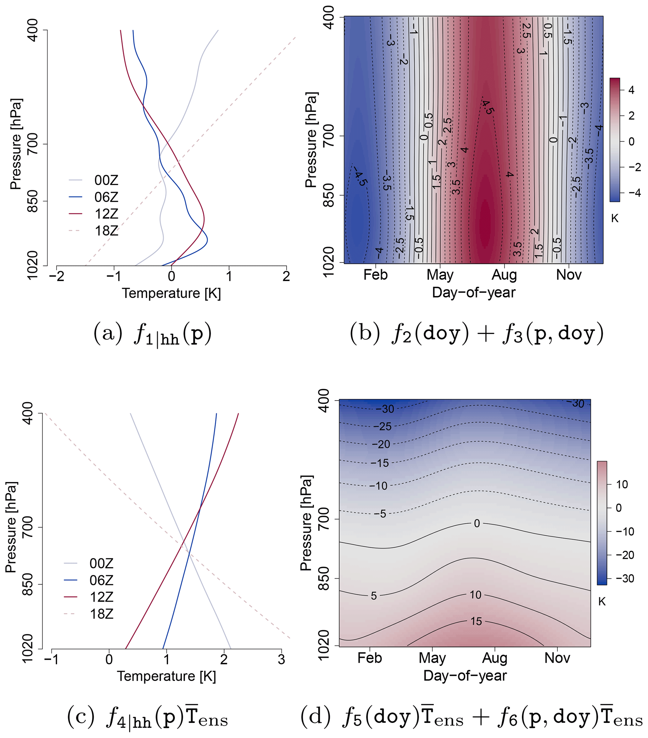
Figure 1Example of the effects of the location parameter μ (Eq. 2) of the NGRVC model for station Bergen. (a) and (b) are the terms of the varying intercept and (c) and (d) the terms of the varying coefficient in Eq. 2 multiplied by . They are computed for the average profiles of by p only (a, c) and p, doy and hh= 12:00 UTC (b, d), respectively, and the average of SDens: 1.08 K.
4.1 Univariate postprocessing
4.1.1 NGR with varying coefficients (NGRVC)
Allowing varying coefficients of the NGR makes a diurnally, seasonally and vertically varying correction of the expected value of the Gaussian forecasting distribution of the EPS possible – as described by Eq. (3). Figure 1 illustrates these effects. Panels (a) and (c) show the diurnally varying vertical contributions to the varying intercept and the varying linear coefficient in the model of the location parameter μ. The strongest correction from the intercept of the early morning sounding at 06:00 UTC is in the layer close to the surface, which would increase the strength of the surface-based inversion in the EPS. The intercept term warms the 12:00 UTC sounding in the boundary layer and immediately above and cools the EPS profile somewhat in the middle of the troposphere. However, the intercept term cannot be seen in isolation. The vertical correction of the varying linear coefficient term (Fig. 1c) warms the original EPS profile on average over the whole year, with the strongest warming in the 18:00 UTC evening/early night sounding. Panels (b) and (d) in Fig. 1 show the effects of the seasonally varying corrections fi(doy) and the interaction of seasonal and vertical corrections fj(doy,p) for the average (over the whole year) 12:00 UTC soundings. The intercept correction adds the seasonal cycle, with the strongest variations in the boundary layer. The seasonally changing correction of the linear term, on the other hand, is less pronounced, especially above the boundary layer, and thus only linearly depends on the ensemble sample variance SDens.
4.1.2 Climatology for SAMOS
SAMOS, a further extension to NGR, makes it possible to correct all vertical levels with one postprocessing model, but requires climatologies of expected value and standard deviation in order to compute the prerequisite standardized anomalies (cf. Sect. 3.2). They were computed with 3 years of observational and NWP data within the mathematical framework of GAMLSS (Sect. A) and the model specification in Eq. (5).

Figure 2Effects of the climatology of observations y for station Bergen (a, b) for the terms f1|hh(p) (hh= 06:00 and 18:00 UTC, respectively, with fixed doy=180) and the combined effects of (for hh= 06:00 UTC); (c) is the standardized anomalies of Tobs used in the SAMOS approach and (d) the quantile–quantile plot of (c) against an idealized Gaussian distribution with an idealized straight solid line.
The effects of the climatology for response Tobs are given in Fig. 2. f1|hh(p) dominates the climatology by capturing the diurnal cycle at the surface (Fig. 2a). Figure 2b shows that the seasonality and the seasonality by pressure have a positive effect in summer and a negative effect in winter and that the amplitude is strongest at the surface. The model thus adds the most temperature to the expected value μ in Eq. (A1) in summer and subtracts the most in the winter season. An n= 10 000 random sample of the standardized anomalies of Tobs (derived from the climatology) is plotted in Fig. 2c. The sample mean and standard deviation (0.01; 1.00) are almost identical to the mean and standard deviation (0; 1) of a standard Gaussian distribution. The line structure in Fig. 2c originates from the model levels of the ECMWF-EPS onto which we interpolate vertically. The quantile–quantile plot in Fig. 2d compares the standardized anomalies in Fig. 2c with the standard Gaussian distribution. The assumption of the Gaussian distributed air temperature is valid but not perfect in the tails beyond 2 sigma.
A climatology is also computed for the ensemble forecasts. The climatology of the ensemble mean is modeled with a single GAMLSS. The standardized anomalies of are similar to those of the observations in Fig. 2c. A simpler approach is sufficient for SDens, which is standardized with the standard deviation of the difference of and the expected value of the climatology, instead of a GAMLSS model for SDens, in agreement with the findings in Dabernig et al. (2017).
4.1.3 SAMOS
Climatological values for mean and standard deviation from Sect. 4.1.2 are then used to standardize the response variables by subtracting the mean and then dividing by the standard deviation, which yields the standardized anomalies , and . This standardization removes most of the pressure-level specific information so that the simplest version of NGR (Eq. 2, with instead of and for SDens) can be applied simultaneously to all pressure levels, seasons and times of (radiosonde) ascent. Corrections for the expected values are fairly small. Using station Bergen as an example, the coefficients of the standard anomaly Eq. (2) are β0=0.0016 (0.0007, 0.0025) and β1=0.9325 (0.9316, 0.9333). Since the intercept is almost zero, basically no offset correction has to be applied. A linear coefficient of less than 1 means that larger values of the standardized anomalies are corrected less than values close to the climatological mean. The respective coefficients for the standardized anomaly of the (log) of the standard deviation are (−1.7966, −1.7877) and γ1=2.0677 (2.0546, 2.0808), respectively. Consequently, a substantial offset correction has to be applied and larger deviations from the climatological mean of the ensemble variance are more strongly corrected.
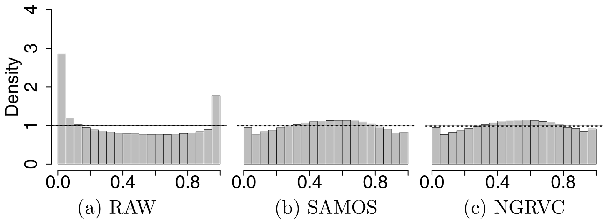
Figure 3PIT histograms of the probability distributions of the raw ensemble (a) and the ensemble postprocessed with SAMOS (b) and the NGRVC (c) for all stations combined. Solid horizontal lines show perfect calibration and the dotted lines are the 95 % consistency interval thereof.
4.1.4 Comparison of calibration and sharpness
Several verification measures are used to compare calibration and sharpness of the distributions resulting from univariate postprocessing with SAMOS and NGRVC, respectively. Calibration is first evaluated with PIT histograms. Figure 3 shows a U shape for the raw ensemble, indicative of a strong underdispersion with truth too frequently beyond the extremes of the forecast. Both SAMOS and NGRVC are better calibrated although slightly overdispersive. The shape might indicate a misspecification of the underlying parametric distribution and possibly skewness (Gebetsberger et al., 2018, 2019).
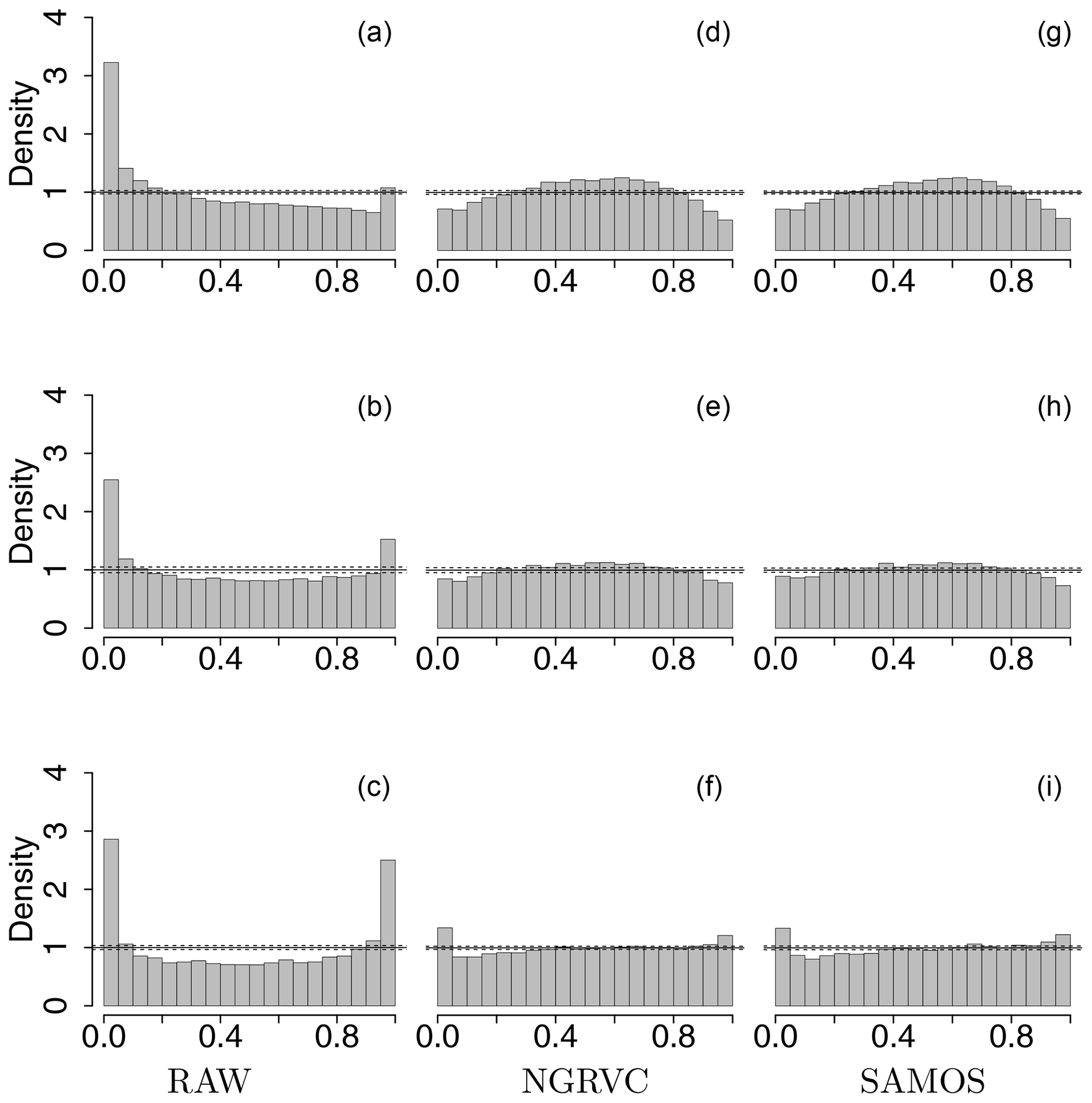
Figure 4PIT histograms by pressure ranges for the probability distributions of the raw ensemble (left), the NGRVC-postprocessed ensemble (middle) and the SAMOS-postprocessed ensemble (right). Bottom row 1020–850 hPa, middle row 850–700 hPa and top row 700–400 hPa for all stations and all launch times combined. Solid horizontal lines show perfect calibration and the dotted lines are the 95 % consistency interval thereof.
Figure 4 zooms into three vertical layers. The strongest underdispersion of the raw ensemble and thus the largest improvement from postprocessing occurs in the lowest layer, 1020–850 hPa, occupied mostly by the planetary boundary layer. The postprocessing of NGRVC and SAMOS cannot completely eliminate the underdispersion in the PIT histogram, which is computed out-of-sample. Deviations of the raw ensemble from the truth are rarer above the boundary layer in the layers 850–700 hPa and 700–400 hPa, where postprocessing effectively removes a cold bias. Overall, the two different approaches of NGRVC and SAMOS have similar PIT histograms at the respective vertical layers.
After calibration the predictive distributions slightly lose sharpness: Fig. 5 shows this increase for widths of the central prediction intervals of 50 % and 90 % (cf. Gneiting and Raftery, 2007), respectively. SAMOS and NGRVC have approximately the same average widths. However, postprocessing reduces the number of times that the prediction interval is extremely (and most likely unnecessarily) wide, as the reduction in the width of the interquartile range and the whiskers from bootstrapping indicate. Additionally, the widths are still only about one-fourth of the width of the interval from the SAMOS climatology (dashed line), which is fitted as a function of time of day, season, pressure level and seasonally varying pressure levels. If one looks at overall verification scores over all four stations, all vertical levels and all times in Table 1, SAMOS considerably improves the log-likelihood and the CRPS, upon which NGRVC improves further. Due to this slight advantage, the NGRVC-postprocessed ensemble is used in the following multivariate postprocessing.
Table 1Out-of-sample negative logarithm of the likelihood (LS) and CRPS of the raw ensemble (RAW), SAMOS and NGRVC probability distributions for all stations combined. Numbers in brackets give the 5th and 95th percentiles of the bootstrapped scores; they represent the 90 % confidence intervals. Bold font indicates the models that performed best.
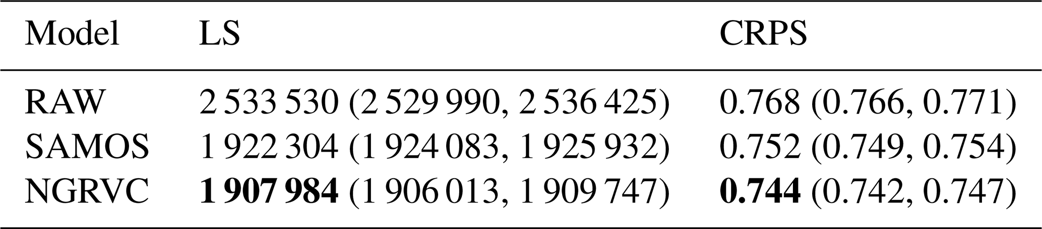
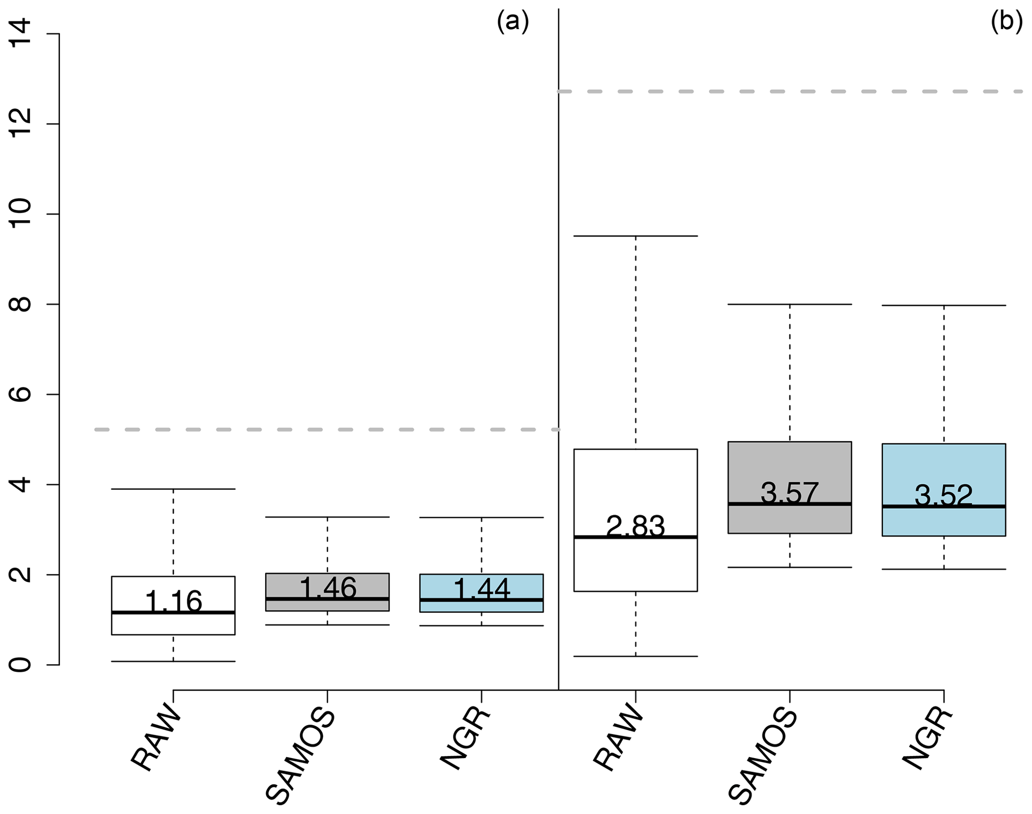
Figure 5Boxplots of the widths of prediction intervals of 50 % (a) and 90 % (b), respectively, from bootstrapping probability distributions of RAW, SAMOS and NGRVC for all stations combined with the value of the median given. The dashed lines mark the respective interval widths of the SAMOS climatology.
4.2 Multivariate postprocessing
Ensemble copula coupling (Sect. 3.3) is used to restore the vertical correlation structure of the temperature profiles contained in the raw ensemble to the univariately corrected temperatures at each level. To better understand the three methods for sampling from the raw ensemble (ECC-Q, ECC-R, ECC-T), they are first demonstrated with two case studies before their forecast performance is evaluated for the whole data set.
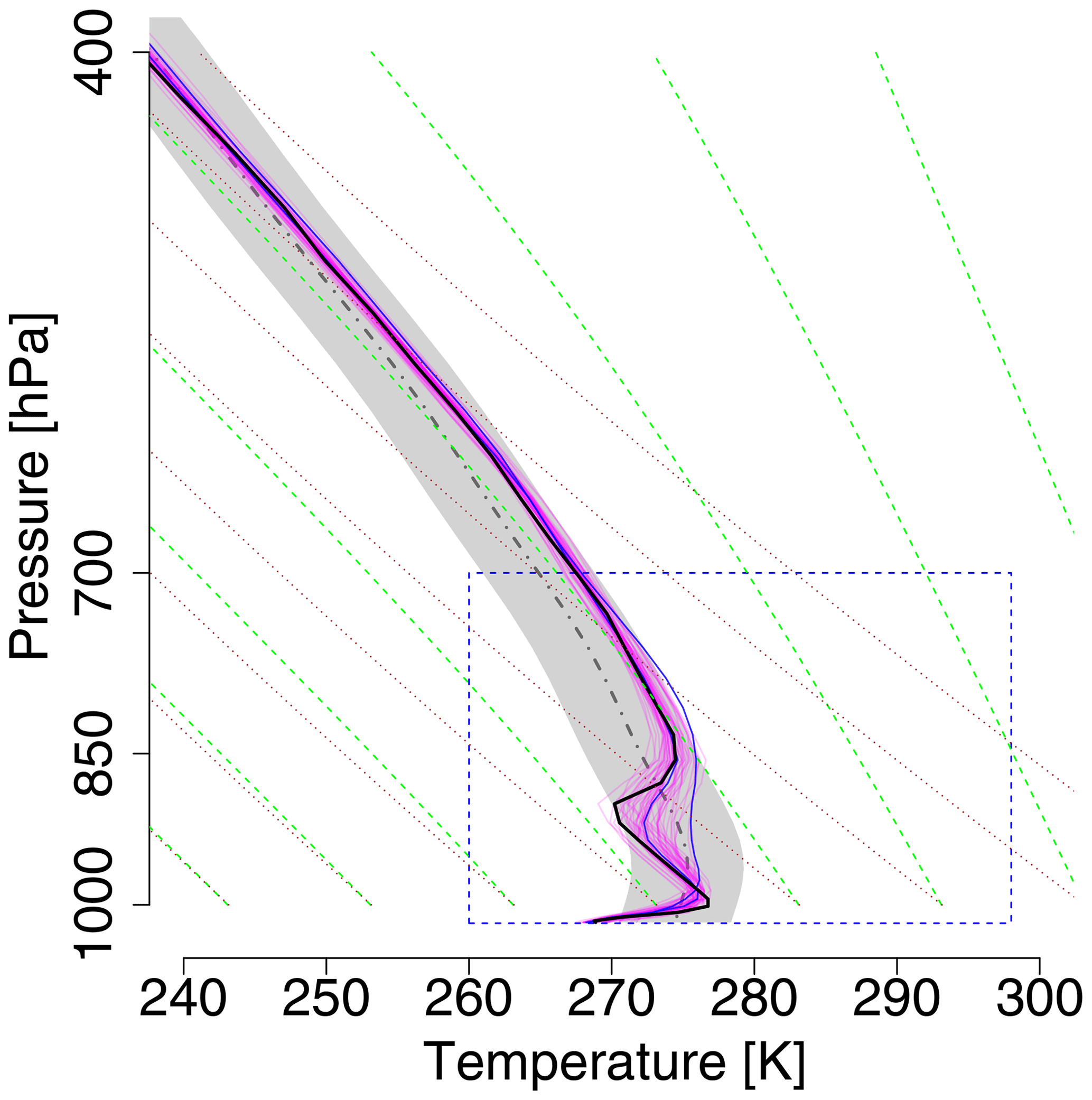
Figure 6Vertical temperature profiles as observed (black bold solid line) and the members (magenta) of the +30 h raw ensemble forecast at station Bergen for 6 December 2016, 06:00 Z. Two members are highlighted with blue. The rectangle with a blue dashed border indicates the zoomed pressure and temperature range plotted in Fig. 7. Gray-thick-dashed-dotted area is the climatological mean of the EPS for this specific date and time and the gray shaded area indicates its ±1 standard deviation range. Green dashed lines are the saturated adiabats, dotted lines the dry adiabats.
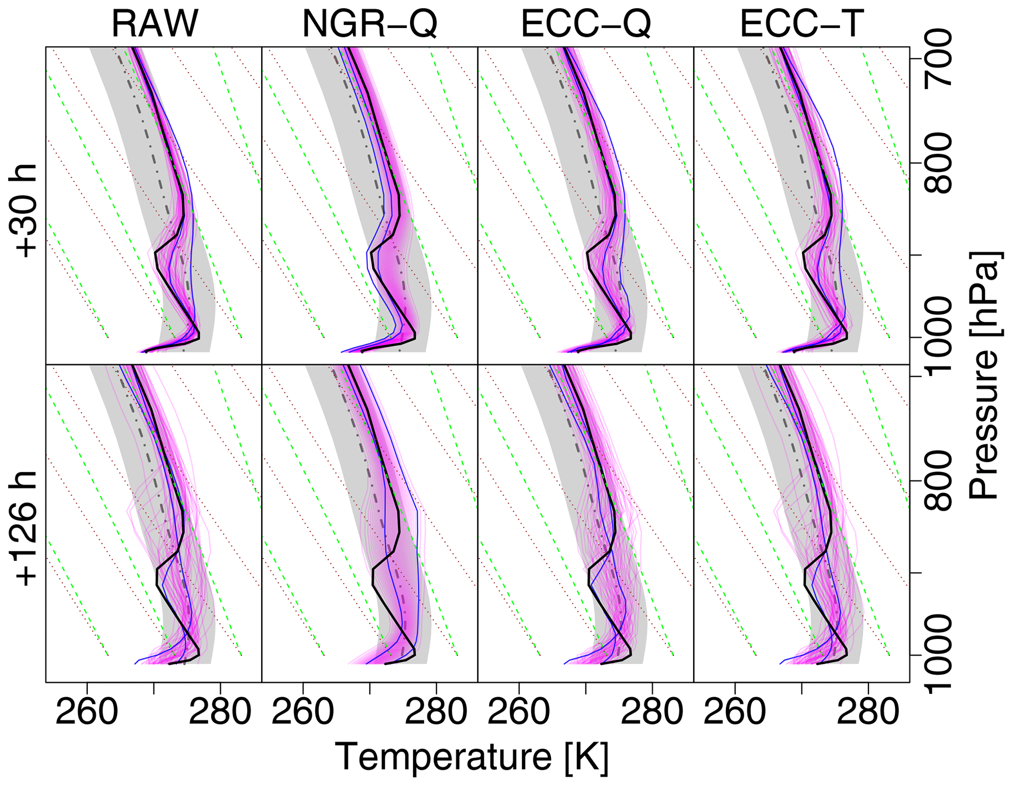
Figure 7Zoom into the rectangle of Fig. 6 with additional postprocessed temperature profiles. The columns show (from left to right) raw ensemble; univariate postprocessing with NGRVC; and multivariate postprocessing with ensemble copula coupling (ECC) of the NGRVC-postprocessed ensemble using quantile sampling (ECC-Q) and distance-preserving sampling (ECC-T), respectively. All figures additionally have observation (bold black), climatological observation (mean (dashed gray) and standard deviation (gray)), and two particular forecast members. The first row contains the forecasts for lead time +30 h, the second row for +126 h.
4.2.1 Case studies
The two case studies show ensemble copula coupling at work in typical winter and summer settings, respectively. The winter morning case is characterized by a strong surface-based temperature inversion, topped by a dry-adiabatically stratified layer, which is capped by a second inversion, as shown by the radiosonde measurements (bold black line) in Fig. 6. All members of the +30 h raw ensemble forecast (magenta solid lines) capture the surface-based inversion, albeit at different altitudes and with different strengths. The spread of the ensemble members around the second inversion is much larger – up to 7 K – and a substantial number of members have only a stable layer but no inversion. Further aloft all members stay within a few degrees of one another and of the observed profile. Figure 7 shows the performance of the postprocessing methods with a zoom into the lower part of the atmosphere where the raw ensemble members have larger deviations. The forecast performance of the raw ensemble deteriorates considerably when the forecasting horizon is extended by another 4 d from +30 to +126 h (second row in Fig. 7). The larger overall spread among the ensemble members indicates the typical increase in forecast uncertainty with forecasting horizon. Especially the second inversion is poorly forecast – either not at all or at different altitudes and/or of different strength – and the spread of the ensemble members is as large as the 2-σ range of the observation climatology, which is indicated by the gray shading.
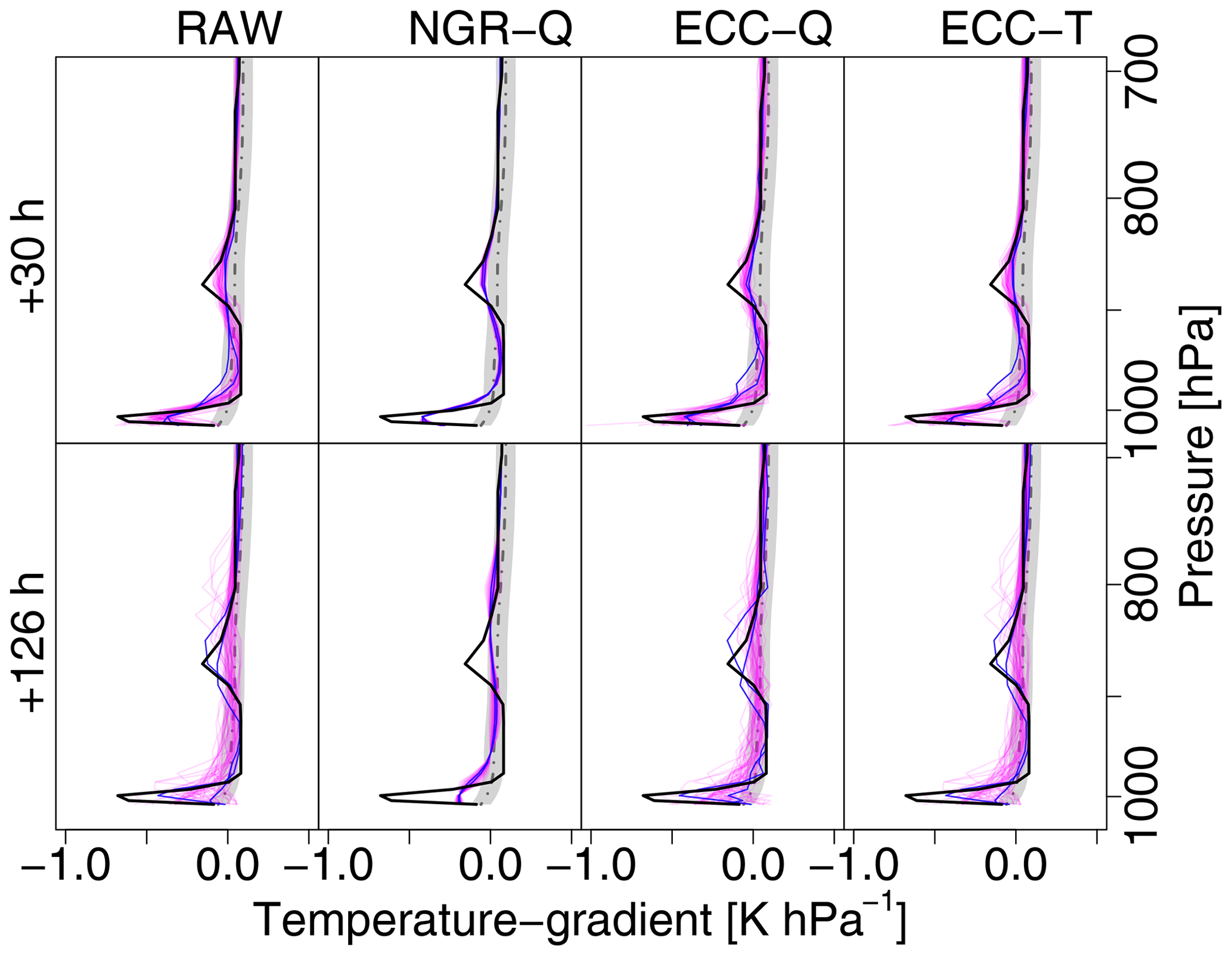
Figure 8Observation (black bold solid) and forecasts (magenta) of the vertical temperature gradient for the 6 December 2016, 06:00 Z winter case. Top row is for lead time +30 h and bottom row for +126 h. Columns show (from left to right) raw ensemble, univariate NGRVC-Q, multivariate ECC-Q and multivariate ECC-T. The same two particular members are highlighted in blue in all the subfigures. Note that a negative temperature gradient in pressure coordinates means an increase in temperature with altitude.
How well do the different methods correct the raw profiles? The univariate NGRVC method (second column of Fig. 7) describes the ensemble members parametrically with a Gaussian distribution and thus corrects only the ensemble mean and standard deviation as a function of the date (here fixed at 6 December 2016, 06:00 Z) and pressure level. Consequently all profiles are parallel to each other. The profiles of two exemplary ensemble members in the +126 h forecast no longer cross as they do in the raw ensemble. Also, the sharpness of the inversions in individual ensemble members is lost when the ensemble mean is formed since they are at different altitudes. However, the spread among individual members might still vary considerably with altitude since it is corrected separately (cf. Sect. 3.1), as is most obvious at the second inversion for the +126 h forecast.
The multivariate ensemble copula coupling method with sampling from the quantiles of the raw ensemble (ECC-Q) restores the overall shape of the member profiles and thus allows the cross-over near the surface of the blue lines in the +126 h forecast. It does not preserve the altitude-dependent spread. For example, the spread above the observed second inversion is reduced considerably by ECC-Q, which effectively eliminates the second inversion from some members. The ensemble copula coupling with distance-preserving correction (ECC-T), on the other hand, keeps the large uncertainty above the observed second inversion. Its corrections are slight, on the order of 1 K over the whole profile.
The vertical temperature gradient determines how easily an air parcel can be displaced in the vertical, which in turn determines exchange processes of, e.g., pollutants and the formation of clouds. Figure 8 shows this gradient, which is the first vertical derivative of the sounding profiles in Fig. 7. Although it is not the response variable of the postprocessing and fitting a model directly to the temperature gradients would likely yield better results, postprocessing should ideally still preserve gradients. The observations (bold lines) show an extremely large gradient in the approximately 30 hPa (300 m) above the surface, which strongly dampens vertical exchange processes. Another albeit weaker such layer is at around 880 hPa. All members of the raw ensemble show the surface-based extremum in a range between a third to the whole observed value. All members also contain the higher-level extremum with only small differences among the members albeit at only half the observed value. Most of the ensemble members of the NWP forecast computed 126 h prior to the observations still capture the strong gradient at the surface. Interestingly a substantial number of members capture the magnitude and depth of the strong gradient further aloft but with a wide range of its location, which is between 900 and 760 hPa. The univariate NGRVC correction (second column in Fig. 8) shifts all members towards a mean value and thus fails to show the larger variation of the temperature gradient. NGRVC only corrects the expectation and the scale of the ensemble, but not members individually. Most of the correction is to the mean. The scale correction is small and varies little over the whole profile, so that the gradient remains nearly the same. Both ensemble copula coupling methods, ECC-Q and ECC-T, on the other hand, bring back the uncertainty of the raw ensemble. For the shorter-term forecast of +30 h, the ECC postprocessing enhances the uncertainty at the lower and upper ends of the extrema of the gradients, while it reduces it (by less) for the longer +126 h forecast – more so for ECC-Q than for ECC-T, which can easily be seen in the two exemplary members (blue lines) of the +126 h forecast.
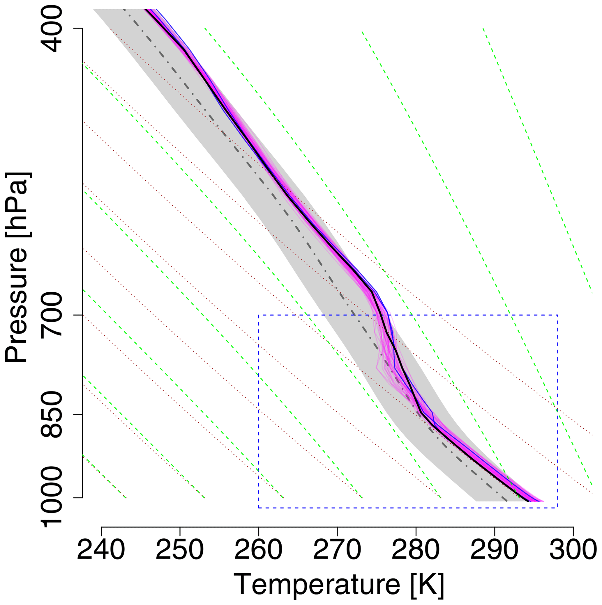
Figure 9As in Fig. 6 but for a summer case of 2 June 2017, 12:00 Z and a lead time of +36 h.
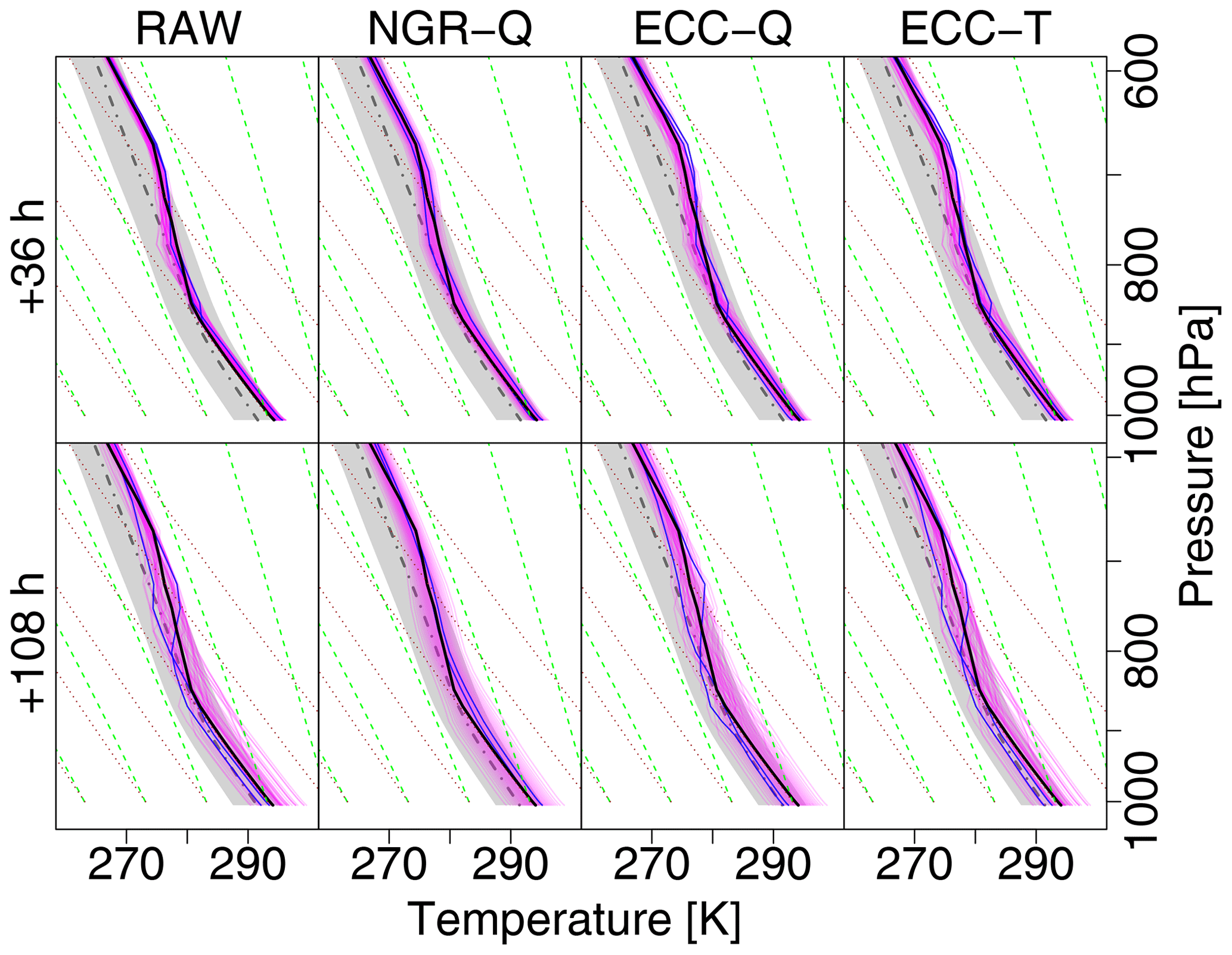
Figure 10As in Fig. 7 but for a summer case of 2 June 2017, 12:00 Z and lead times of +36 h (first row) and +108 h (second row), respectively.
The second case study of a summer noon profile exemplifies the performance for a deep convective boundary layer capped by a thick stable layer and a nearly moist-adiabatic stratification aloft where the profile parallels the green saturated adiabat in Fig. 9. In contrast to the winter case, forecast uncertainty is much lower; the spread of the ensemble members within the boundary layer in the +36 h forecast is only a fraction of the 2-σ range of the climatological profile (gray shading) and still less than that range for the +108 h forecast as seen in Fig. 10. Similarly to the winter case, the spread above the top of the boundary layer is only about 1 K, and the observation lies within the range of the forecast. Since the univariate NGRVC method only corrects ensemble mean and standard deviation thin stable layers in individual ensemble members at the top of their respective surface-based convective boundary layers are not kept and smoothed out. Contrarily, both multivariate ensemble copula coupling methods are naturally able to keep them. As in the winter case, corrections from ECC-T are smaller than from ECC-Q. Without being able to fully explain this behavior, we speculate that this is related to the fact that ECC-Q assumes equally spaced probabilities for the transformation from probability space to temperature space. ECC-T borrows these probabilities from the raw ensemble. Thus, ECC-T could potentially represent outliers better than ECC-Q, as points in probability space can be distinct from the majority of the points.
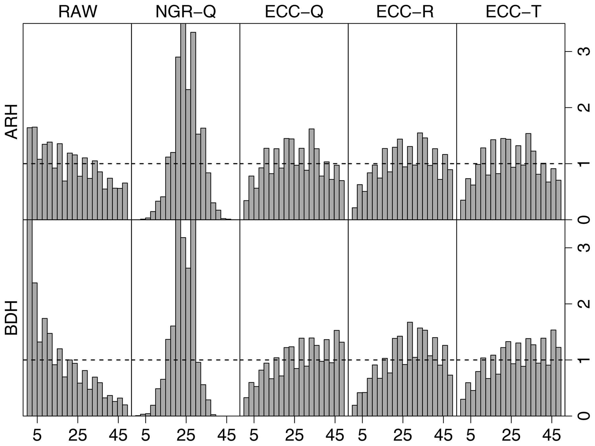
Figure 11Multivariate rank histograms of the samples of the raw ensemble (RAW), quantile sample of the NGRVC-postprocessed ensemble (NGRVC-Q), quantile sample of ECC (ECC-Q), random sample of ECC (ECC-R) and the transformed RAW sample (ECC-T). Top row: average rank histograms; bottom: band-depth histograms. Data include all available stations, all lead times and the 31 pressure levels between 1020 and 400 hPa.
4.3 Evaluation of forecast performance over the whole period
The performance of the different correction methods is evaluated both graphically with rank histograms and numerically with the energy score and variogram score (cf. Sect. 3.4) for the whole period 15 September 2016–15 September 2019.
Figure 11 assesses the calibration of forecasts over all locations, lead times and pressure levels graphically through average (ARH) and band-depth (BDH) multivariate rank histograms. The strong excess at low ranks in both histograms suggests that the raw ensemble profiles are systematically too warm. The pronounced ∩ shape of the average rank histogram for the quantile samples of univariate NGRVC correction (second column in Fig. 11) indicates overdispersion. This is due to the construction of the NGRVC-Q ensemble, which assumes a correlation of unity between the temperatures at different levels (Wilks, 2017). All three versions of the multivariate ensemble copula coupling reduce this overdispersion, but fail to eliminate it.
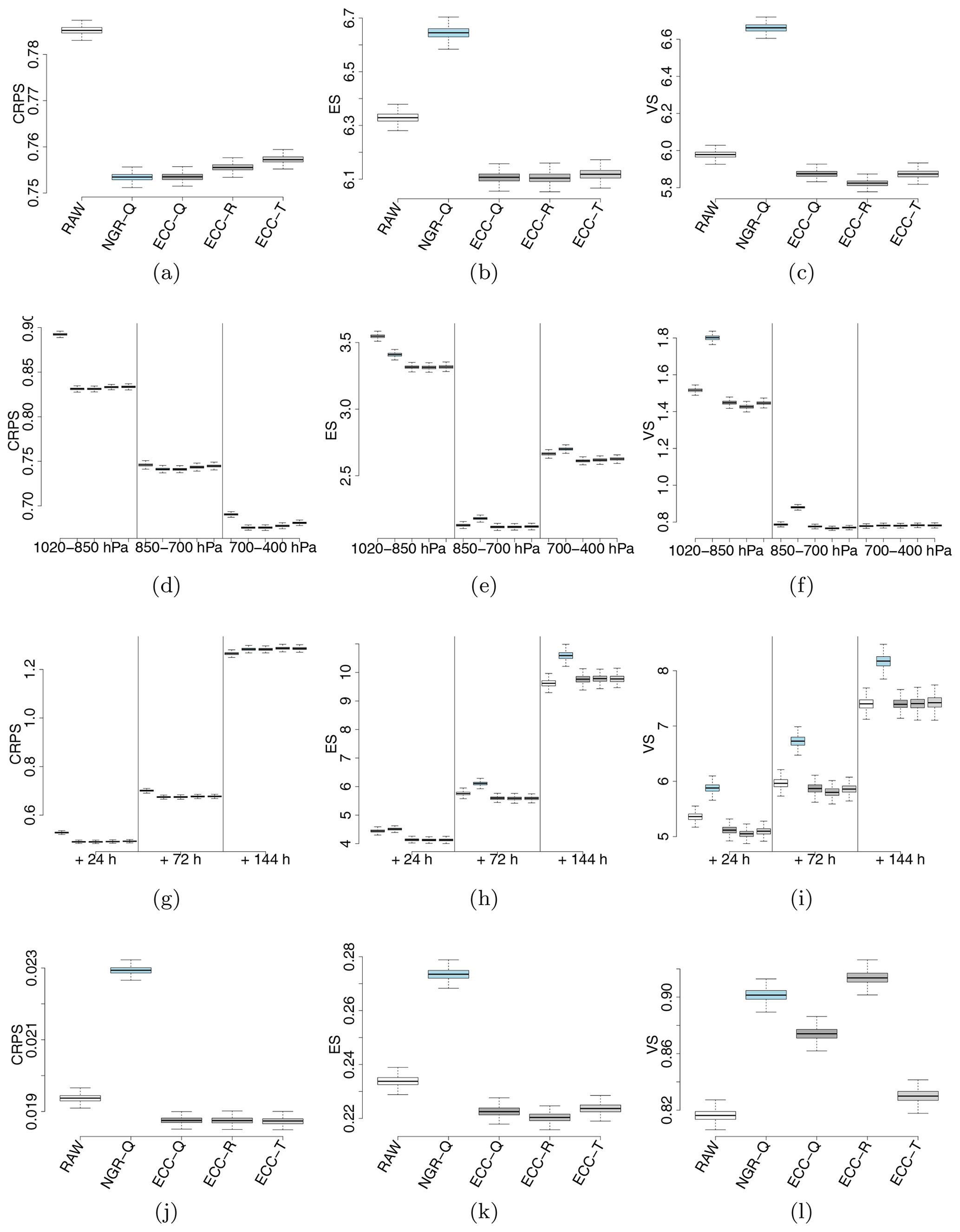
Figure 12Bootstrapped continuous ranked probability score (CRPS, first column), energy score (ES, second column) and variogram score (VS, third column) for the raw ensemble (RAW), the quantile sample of the NGR-postprocessed (NGRVC-Q), the quantile sample of ECC (ECC-Q), the random sample of ECC (ECC-R) and the transformed sample of ECC (ECC-T). The first row shows results for all pressure ranges and lead times combined, the second row stratified by three pressure ranges but over all lead times, and the third row by three lead times. Note that the range of the scores changes between rows. The bottom row shows the scores for the temperature gradient dT∕dp. Lower values are better for all three scores.
Figure 12 shows the univariate performance as evaluated with the CRPS (first column) and compares it to the multivariate performance evaluated with the energy score, which is the multivariate generalization of the CRPS (second column), and with the variogram score, which weights the representation of the correlation structure more strongly (third column). Lower values of all three scores are better. When evaluated over all lead times and vertical levels (first row) the univariate metric of the CRPS score in Fig. 12 obviously shows the largest improvement for the univariate postprocessing method (NGR-Q). However, the CRPS score for the multivariate ensemble copula coupling methods is on par or only slightly worse. When the multivariate metrics of energy score (Fig. 12a) and variogram score (Fig. 12c) are used, the univariate one falls decisively behind even the raw ensemble, as already seen in the rank histograms (Fig. 11) and the winter case study (Fig. 8).
When the scores are stratified into three pressure ranges (second row of Fig. 12) it can be seen in all three metrics that the lowest layer next to the surface is the most difficult one for the raw ensemble. However, this is also the layer where the postprocessing achieves the largest improvements in all three scores. Unsurprisingly, the univariate postprocessing has poorer multivariate metrics of energy and variogram scores than the raw ensemble (with the exception of the energy score of the lowest layer). Improvements from the copula coupling methods in the lowest layer are much larger than in the two layers higher up. One result for which we have no explanation is why the energy score of the raw ensemble is better for the layer between 850 and 700 hPa, which is still partly in the boundary layer for at least part of the times, than for the layer above the altitude of the 700 hPa level. The variogram score, which more strongly weights the structure of the profile, does not show such a behavior.
A stratification by lead time (third row of Fig. 12) shows first the expected worsening of the raw ensemble scores for longer lead times. Again, the multivariate scores of the univariately postprocessed (NGR-Q) ensemble are worse than for the raw ensemble. While the copula coupling methods still improve the raw ensemble for a +72 h forecast, 144 h are too far into the future to still achieve an improvement over the raw ensemble data.
The last row of Fig. 12 shows the vertical temperature gradient, which is only a derived quantity but not the response variable of the postprocessing itself. Therefore it should not come as a surprise that the univariate postprocessing with NGR-Q performs worse than the raw ensemble for the univariate CRPS metric. The copula coupling methods manage to improve the energy score over the raw ensemble. However, they cannot beat the raw ensemble in the variogram score. Since the variogram score weights the correlation aspect of the multivariate performance more strongly, this indicates that if one is interested in accurate temperature gradient forecasts it might be advisable to directly postprocess the gradients themselves instead of deriving them from the postprocessed temperatures.
Postprocessing ensembles of numerical weather prediction model forecasts with statistical models trained on past ensemble forecasts and “truth”, i.e., observations, improves these forecasts further and has thus been a burgeoning field of research, of which Vannitsem et al. (2018) give a comprehensive review. A recent push has been towards multivariate postprocessing, which honors the correlation structure – be it between different variables or the same variable along time or in space. One popular method is copula coupling. When applied in space, the method has so far been limited to (quasi)-horizontal data, e.g., air temperature at three sites (three dimensions) (Schefzik, 2017) or (quasi)-horizontal fields of temperature, precipitation and wind (Schefzik et al., 2013).
Postprocessing the vertical structure of (ensemble) NWP forecasts, however, has remained largely unexplored. Since the vertical structure strongly influences exchange processes, onset and cessation of convection, formation of clouds and precipitation, improvement over the raw ensemble forecasts is arguably as important as for horizontal fields. Renkl (2013) started to explore the potential by postprocessing vertical temperature profiles from EPS forecasts by combining a reduction of the dimensionality with kriging. He reduced the dimensions of the vertical profiles by reconstructing them with their leading normal modes, which retained about 80 % of their variance. Subsequently the coefficients of these modes were adjusted with kriging for groups of ensemble members.
We take a different approach modeled on results for quasi-horizontal postprocessing and postprocess the vertical profiles using a combination of univariate calibration and copula coupling. ECC needs probability distributions, also known as margins, at each pressure level. The margins are obtained by two univariate techniques, which are enhanced variants of the classical nonhomogeneous Gaussian regression (NGR). When the coefficients of NGR vary diurnally, seasonally and in the vertical (NGRVC, Simon et al. (2017); Lang et al. (2020)) the performance is slightly better than when using standardized anomalies with precomputed diurnally, seasonally and vertically varying climatologies of the SAMOS approach (Dabernig et al., 2017; Stauffer et al., 2017). While NGRVC was used here for preprocessing the data for ECC, SAMOS is equally suitable. NGRVC only corrects the expectation and the scale of the whole ensemble, but not of members individually. If the scale correction varies little over the whole profile, as is the case here, the vertical gradient remains nearly the same, which might be a disadvantage when achieving strongly varying gradients is important for the further application of the postprocessed profiles.
Stable layers, for example, are crucial for the impediment of vertical motions and exchange: they determine the top of the boundary layer and the mixing volume for pollutants. While their scale might be too small to have predictability to +6 d, the processes forming them such as surface heating and large-scale subsidence might still be predictable. For a forecaster it is important to know about the possible existence of (very) stable layers despite an uncertainty in altitude, thickness and strength instead of having to infer their existence from a slight increase in stability in a smoothed-out profile that a univariate postprocessing such as NGRVC delivers.
Using the univariately corrected margins for further and multivariate postprocessing with copula coupling better reproduces such (potentially very thin) stable layers. With ECC the rank order structure of the ensemble of NWP forecasts from the ECMWF-EPS is conserved. Several sampling strategies might be used with copula coupling. We used three. To sample randomly (ECC-R) is unadvisable as it may deliver worse results than the raw ensemble forecasts. On the other hand, quantile resampling (ECC-Q) and sampling with rescaling of the raw ensemble by conserving the relative distances between ensemble members (ECC-T) and thus also accounting for extreme ensemble members are successful. Of the two, ECC-T is overall better than ECC-Q in all three verification measures used: rank histograms, energy score and variogram score.
The largest improvements are obtained for the profiles in the atmospheric boundary layer over all lead times and all seasons and also in the two case studies shown. Consequently, this is also the layer where the largest potential for improvements of the NWP model is, which is a well-known fact (e.g., Holtslag et al., 2013) since many processes shaping the boundary layer have to be parameterized in such models. The current postprocessing approach has potential for further improvement by adding more covariates, as has been shown in other postprocessing scenarios (e.g., Scheuerer, 2014; Scheuerer and Hamill, 2015a; Messner et al., 2017). For some practical forecasting purposes, the humidity forecasts have to be additionally postprocessed with the constraint that the dew-point temperature must not exceed the (dry-bulb) temperature.
The main motivation for using GAMLSS models is to be able to set up additive predictors of nonlinear smooth functions for each parameter of a distribution (Rigby and Stasinopoulos, 2005).
We assume that the response variable y follows a parametric probability distribution 𝒟, which is determined by k parameters θ1, θ2, …, θk:
The parameters θ1, θ2, …, θk determine the location, scale and shape of the probability distribution. The parameters are conditioned on covariates in a nonlinear way by additive predictors such as
which can be set up for each parameter and where g(⋅) is a link function that maps the parameter to the real line. For instance, for a Gaussian distribution μ and σ are linked to their predictors using the identity and the log function, respectively, for g(⋅). The latter ensures that the parameter σ is strictly positive, while its predictor can take any value on the real line.
The functional terms f⋆ in Eq. A2 are modeled by spline bases such as thin plate or cyclic cubic splines (Wood, 2017). They are employed within the additive predictor in various forms.
-
f1(x1) is a one-dimensional smooth, potentially nonlinear function depending on the covariate x1.
-
f2(x2,x3) is a two-dimensional smooth function based on the tensor product of two univariate spline bases that depends on the covariates x2 and x3.
-
f3(x4)⋅x5 expresses a linear relationship of x5 with a varying coefficient expressed by the smooth function f3(x4) depending on x4.
In the present study GAMLSS models are estimated by maximizing a penalized log-likelihood. The models were fitted with R package gamlss (Stasinopoulos and Rigby, 2007).
ECMWF-EPS data of ensemble mean and standard deviation used for univariate postprocessing are available from ECMWF upon request. Charges may apply. Data at model levels of individual ensemble members, which ECMWF does not store, are available from the authors after receiving permission from ECMWF (ECMWF, 2012). Radiosonde data are freely available from the Integrated Global Radiosonde Archive (IGRA, NOAA, 2019).
Data were processed in R using the following packages: mgcv, gamlss, crch and scoringRules.
DS, TS, GJM defined the scientific scope of this study. DS performed the statistical modelling and evaluated the results. GJM supported the meteorological analysis. TS contributed to the development of the statistical methods. All the authors contributed to the paper by writing significant parts. Furthermore all the authors discussed the results and commented on the manuscript.
The authors declare that they have no conflict of interest.
We thank the editor Chris Forest and four anonymous referees for their efforts.
This research has been supported by the Austrian Research Promotion Agency (FFG) (grant no. 846620) and the Austrian Science Fund (FWF) (grant no. P31836).
This paper was edited by Chris Forest and reviewed by four anonymous referees.
Blandford, T. R., Humes, K. S., Harshburger, B. J., Moore, B. C., Walden, V. P., and Ye, H.: Seasonal and Synoptic Variations in Near-Surface Air Temperature Lapse Rates in a Mountainous Basin, J. Appl. Meteorol. Climatol., 47, 249–261, https://doi.org/10.1175/2007JAMC1565.1, 2008. a
Dabernig, M., Mayr, G. J., Messner, J. W., and Zeileis, A.: Spatial ensemble post-processing with standardized anomalies, Q. J. Roy. Meteor. Soc., 143, 909–916, https://doi.org/10.1002/qj.2975, 2017. a, b, c, d, e
Durre, I., Vose, R. S., and Wuertz, D. B.: Robust Automated Quality Assurance of Radiosonde Temperatures, J. Appl. Meteorol. Climatol., 47, 2081–2095, https://doi.org/10.1175/2008JAMC1809.1, 2008. a
ECMWF: Describing ECMWF’s forecasts and forecasting system, ECMWF Newsletter, 133, 11–13, 2012. a, b
Gebetsberger, M., Messner, J. W., Mayr, G. J., and Zeileis, A.: Estimation Methods for Nonhomogeneous Regression Models: Minimum Continuous Ranked Probability Score versus Maximum Likelihood, Mon. Weather Rev., 146, 4323–4338, https://doi.org/10.1175/MWR-D-17-0364.1, 2018. a
Gebetsberger, M., Stauffer, R., Mayr, G. J., and Zeileis, A.: Skewed logistic distribution for statistical temperature post-processing in mountainous areas, Adv. Stat. Clim. Meteorol. Oceanogr., 5, 87–100, https://doi.org/10.5194/ascmo-5-87-2019, 2019. a
Gneiting, T. and Raftery, A. E.: Weather forecasting with ensemble methods, Science, 310, 248–249, https://doi.org/10.1126/science.1115255, 2005. a
Gneiting, T. and Raftery, A. E.: Strictly proper scoring rules, prediction, and estimation, J. Am. Stat. Assoc., 102, 359–378, https://doi.org/10.1198/016214506000001437, 2007. a, b, c
Gneiting, T., Raftery, A. E., Westveld III, A. H., and Goldman, T.: Calibrated probabilistic forecasting using ensemble model output statistics and minimum CRPS estimation, Mon. Weather Rev., 133, 1098–1118, https://doi.org/10.1175/MWR2904.1, 2005. a, b, c, d, e
Gneiting, T., Balabdaoui, F., and Raftery, A. E.: Probabilistic forecasts, calibration and sharpness, J. R. Stat. Soc. B, 69, 243–268, https://doi.org/10.1111/j.1467-9868.2007.00587.x, 2007. a, b
Hagedorn, R., Buizza, R., Hamill, T. M., Leutbecher, M., and Palmer, T. N.: Comparing TIGGE multimodel forecasts with reforecast-calibrated ECMWF ensemble forecasts, Q. J. Roy. Meteor. Soc., 138, 1814–1827, https://doi.org/10.1002/qj.1895, 2012. a
Hersbach, H.: Decomposition of the continuous ranked probability score for ensemble prediction systems, Weather and Forecasting, 15, 559–570, https://doi.org/10.1175/1520-0434(2000)015<0559:DOTCRP>2.0.CO;2, 2000. a
Holtslag, A. A. M., Svensson, G., Baas, P., Basu, S., Beare, B., Beljaars, A. C. M., Bosveld, F. C., Cuxart, J., Lindvall, J., Steeneveld, G. J., Tjernström, M., and Wiel, B. J. H. V. D.: Stable atmospheric boundary layers and diurnal cycles: Challenges for weather and climate models, B. Am. Meteorol. Soc., 94, 1691–1706, https://doi.org/10.1175/BAMS-D-11-00187.1, 2013. a, b, c
Jordan, A., Krüger, F., and Lerch, S.: Evaluating Probabilistic Forecasts with scoringRules, J. Stat. Softw., 90, 1–37, https://doi.org/10.18637/jss.v090.i12, 2019. a
Lang, M. N., Lerch, S., Mayr, G. J., Simon, T., Stauffer, R., and Zeileis, A.: Remember the past: a comparison of time-adaptive training schemes for non-homogeneous regression, Nonlin. Processes Geophys., 27, 23–34, https://doi.org/10.5194/npg-27-23-2020, 2020. a, b, c
Markowski, P. and Richardson, Y.: Mesoscale meteorology in midlatitudes, Wiley-Blackwell, https://doi.org/10.1002/9780470682104, 2010. a
Messner, J. W., Mayr, G. J., and Zeileis, A.: Non-homogeneous boosting for predictor selection in ensemble postprocessing, Mon. Weather Rev., 145, 137–147, https://doi.org/10.1175/MWR-D-16-0088.1, 2017. a
NOAA: NOAA Integrated Global Radiosonde Archive (IGRA), available at: https://www.ncdc.noaa.gov/data-access/weather-balloon/integrated-global-radiosonde-archive, last access: 19 December 2019. a, b
Pinson, P. and Girard, R.: Evaluating the quality of scenarios of short-term wind power generation, Appl. Energ., 96, 12–20, https://doi.org/10.1016/j.apenergy.2011.11.004, 2012. a
R Core Team: R: A Language and Environment for Statistical Computing, R Foundation for Statistical Computing, Vienna, Austria, available at: https://www.R-project.org/ (last access: 19 December 2019), 2019. a
Reeves, H. D., Elmore, K. L., Ryzhkov, A., Schuur, T., and Krause, J.: Sources of Uncertainty in Precipitation-Type Forecasting, Weather Forecast., 29, 936–953, https://doi.org/10.1175/waf-d-14-00007.1, 2014. a
Renkl, C.: The Vertical Structure of the Atmosphere in COSMO-DE-EPS: Multivariate Ensemble Postprocessing in the Space of Vertical Normal Modes, Tech. rep., Rheinische Friedrich-Wilhelms-Universität Bonn, 2013. a, b
Rigby, R. A. and Stasinopoulos, D. M.: Generalized additive models for location, scale and shape, J. R. Stat. Soc. C-Appl., 54, 507–554, https://doi.org/10.1111/j.1467-9876.2005.00510.x, 2005. a, b
Rozanov, V., Rozanov, A., Kokhanovsky, A., and Burrows, J.: Radiative Transfer Through Terrestrial Atmosphere and Ocean: Software Package Sciatran, J. Quant. Spectrosc. Ra., 133, 13–71, https://doi.org/10.1016/j.jqsrt.2013.07.004, 2014. a
Schefzik, R.: Ensemble calibration with preserved correlations: Unifying and comparing ensemble copula coupling and member-by-member postprocessing, Q. J. Roy. Meteor. Soc., 143, 999–1008, https://doi.org/10.1002/qj.2984, 2017. a
Schefzik, R., Thorarinsdottir, T. L., and Gneiting, T.: Uncertainty quantification in complex simulation models using ensemble copula coupling, Stat. Sci., 28, 616–640, https://doi.org/10.1214/13-STS443, 2013. a, b, c, d
Scheuerer, M.: Probabilistic quantitative precipitation forecasting using ensemble model output statistics, Q. J. Roy. Meteor. Soc., 140, 1086–1096, https://doi.org/10.1002/qj.2183/full, 2014. a
Scheuerer, M. and Hamill, T. M.: Statistical postprocessing of ensemble precipitation forecasts by fitting censored, shifted gamma distributions, Mon. Weather Rev., 143, 4578–4596, https://doi.org/10.1175/MWR-D-15-0061.1, 2015a. a
Scheuerer, M. and Hamill, T. M.: Variogram-based proper scoring rules for probabilistic forecasts of multivariate quantities, Mon. Weather Rev., 143, 1321–1334, https://doi.org/10.1175/MWR-D-14-00269.1, 2015b. a, b, c
Simon, T., Umlauf, N., Mayr, G. J., and Zeileis, A.: Boosting Multivariate Gaussian Models for Probabilistic Temperature Forecasts, in: Proceedings of the 32nd International Workshop on Statistical Modelling, Groningen, Netherlands, University of Groningen, 143–148, available at: https://iwsm2017.webhosting.rug.nl/IWSM_2017_V1.pdf (last access: 19 December 2019), 2017. a, b
Simon, T., Fabsic, P., Mayr, G. J., Umlauf, N., and Zeileis, A.: Probabilistic Forecasting of Thunderstorms in the Eastern Alps, Mon. Weather Rev., 146, 2999–3009, https://doi.org/10.1175/MWR-D-17-0366.1, 2018. a
Stasinopoulos, D. and Rigby, R.: Generalized additive models for location scale and shape (GAMLSS) in R, J. Stat. Softw., 23, 1–46, https://doi.org/10.18637/jss.v023.i07, 2007. a
Stauffer, R., Umlauf, N., Messner, J. W., Mayr, G. J., and Zeileis, A.: Ensemble Postprocessing of Daily Precipitation Sums over Complex Terrain Using Censored High-Resolution Standardized Anomalies, Mon. Weather Rev., 145, 955–969, https://doi.org/10.1175/mwr-d-16-0260.1, 2017. a
Thorarinsdottir, T. L., Scheuerer, M., and Heinz, C.: Assessing the calibratio of high-dimensional ensemble forecasts using rank histograms, J. Comput. Graph. Stat., 25, 105–122, https://doi.org/10.1080/10618600.2014.977447, 2016. a
Vannitsem, S., Wilks, D., and Messner, J., eds.: Statistical Postprocessing of Ensemble Forecasts, Elsevier Science, https://doi.org/10.1016/C2016-0-03244-8, 2018. a
Whiteman, C. D., Hoch, S. W., Horel, J. D., and Charland, A.: Relationship Between Particulate Air Pollution and Meteorological Variables in Utah's Salt Lake Valley, Atmos. Environ., 94, 742–753, https://doi.org/10.1016/j.atmosenv.2014.06.012, 2014. a
Wilks, D. S.: Multivariate ensemble model output statistics using empirical copulas, Q. J. Roy. Meteor. Soc., 141, 945–952, https://doi.org/10.1002/qj.2414, 2015. a
Wilks, D. S.: On assessing calibration of multivariate ensemble forecasts, Q. J. Roy. Meteor. Soc., 143, 164–172, https://doi.org/10.1002/qj.2906, 2017. a, b
Wood, S. N.: Generalized Additive Models: An Introduction with R, Texts in Statistical Science, Chapman & Hall/CRC, Boca Raton, 2nd edn., 2017. a