the Creative Commons Attribution 4.0 License.
the Creative Commons Attribution 4.0 License.
 | 16 Apr 2019
Fitting a stochastic fire spread model to data
X. Joey Wang
John R. J. Thompson
W. John Braun
Douglas G. Woolford
As the climate changes, it is important to understand the effects on the environment. Changes in wildland fire risk are an important example. A stochastic lattice-based wildland fire spread model was proposed by Boychuk et al. (2007), followed by a more realistic variant (Braun and Woolford, 2013). Fitting such a model to data from remotely sensed images could be used to provide accurate fire spread risk maps, but an intermediate step on the path to that goal is to verify the model on data collected under experimentally controlled conditions. This paper presents the analysis of data from small-scale experimental fires that were digitally video-recorded. Data extraction and processing methods and issues are discussed, along with an estimation methodology that uses differential equations for the moments of certain statistics that can be derived from a sequential set of photographs from a fire. The interaction between model variability and raster resolution is discussed and an argument for partial validation of the model is provided. Visual diagnostics show that the model is doing well at capturing the distribution of key statistics recorded during observed fires.
- Article
(3081 KB) -
Supplement
(2301 KB) - BibTeX
- EndNote


1.1 The need for wildland fire spread models
The risk of large catastrophic wildland fires appears to be increasing in many countries as evidenced by recent high-profile wildfire events including the 2016 Fort McMurray fire in Canada and the “Black Saturday” bushfires of 2009 in Australia. Of heightened concern are climate change impacts on wildland fires. Weber and Stocks (1998) postulated that increasing temperatures could lead to an increased number of wildland fire ignitions, a longer fire season, and/or an increased number of days with severe fire weather. In regions of Canada, fire seasons are getting longer (Albert-Green et al., 2012) and fire risk has been shown to be increasing (Woolford et al., 2010, 2014). Annual area burned has increased and has been connected to human-induced climate change (Gillett et al., 2004). Studies that analyzed data output from climate model scenarios have suggested increased severity ratings (Flannigan and Van Wagner, 1991), area burned (Flannigan et al., 2005), ignitions (Wotton et al., 2010), and a longer fire season (Wotton and Flannigan, 1993).
Consequently, the development of accurate, spatially explicit fire spread models is of crucial importance for understanding aspects of fire behaviour and forecasting whether and how a wildland fire may spread. Many fire spread models are deterministic and although there have been some efforts to incorporate randomness into such models, there is also a strong need to develop stochastic fire spread models along with the statistical methodology for calibrating such models to data so that the uncertainty associated with where and when a fire might spread can be determined. A well-calibrated fire spread model can be used at the incident level for individual fire management or be coupled to fire occurrence and fire duration models in a simulation-based approach for longer-term strategic planning by wildland fire management agencies.
1.2 An overview and some recent developments
Taylor et al. (2013; Sect. 3) provided a detailed review of fire growth, discussing the physical process of fire growth, fire spread rate models, and spatially explicit fire growth models, including a discussion of deterministic fire spread models, such as Prometheus (Tymstra, 2005) and FARSITE (Finney, 2004), which play important roles in operational fire spread modelling by fire management agencies. Although these simulators are well established and used frequently in Canada, the United States, and in several other countries, their chief weakness is that they are not stochastic. Fire managers would benefit from probability maps to indicate where a currently burning fire may spread.
Burn-P3 (e.g. Parisien et al., 2005) used the deterministic Prometheus fire spread model in an ensemble-type simulation procedure which randomizes weather sequences in order to induce randomness to produce “burn probability maps”, typically a gridded map of the susceptibility of the landscape to be burned by wildfire over a large study area over the course of a year. We note that this kind of procedure may be more appropriate for studying fire risk on large temporal and spatial scales, such as producing an annual burn probability map for a region or district where wildland fires are managed. However, modelling at the incident level, namely quantifying whether or not a given fire may spread and where it may spread to along with estimating the uncertainty associated with the spread of a single fire, requires a different approach.
We note that deterministic models, such as Prometheus, can and are used at the incident level to model the spread of a single fire given local conditions. We also note that there has been some work to incorporate randomness into the Prometheus fire growth engine. For example, Garcia et al. (2008) attempted to introduce stochasticity to the Prometheus model via a block bootstrap procedure, and Han and Braun (2014) incorporated uncertainty through introducing an error component into the underlying model for rate of spread (ROS), as a parametric bootstrap. Nevertheless, much work remains to be done in order to make these procedures operational.
In the meantime, several other models have been considered by several other authors, including the stochastic lattice-spread model of Boychuk et al. (2007) that was studied by Braun and Woolford (2013), who also introduced an interesting variant of that lattice-spread model in their paper. This modified Boychuk model is used in our study herein where we address some statistical issues, studying the model from the point of view of data analysis not through operational implementation, which we illustrate through the analysis of some small experimental fires or “microfires”. We purposely restrict our analysis to such microfire data in order to study the model on data collected under controlled experimental conditions.
1.3 The modified Boychuk fire spread model
We study the modified version of the Boychuk et al. (2007) model as described in Braun and Woolford (2013). In its simplest special case one assumes the landscape to be flat with a fuel type and density that is homogeneous, the weather conditions to be constant, and no wind. On this landscape we impose a regular square n×m lattice. Each of the grid cells can be in one of three possible states: unburned fuel (F), burning fuel (B), or burnt out (O). Transitions between these states occur as follows: initially (i.e. at time t=0), the grid cell at some location (i,j) is in state B, while all other cells are in state F. The fire burning in cell (i,j) will spread to each of its four nearest neighbours (i.e. north, south, east, and west) in random amounts of time and , provided it does not burn out first. Specifically, at time T0,1, the cell at makes the transition from state F to B, if the cell is not already in state B. Similar transitions are made by cell at , cell at T1,0, and cell at . These times are assumed to be independent and exponentially distributed with a mean of 1∕λ. Once a cell has made a transition to state B, fire spreads from that cell to the sites of its nearest neighbourhood at a new set of independent exponential random times. The time until the next burning cell burns out is exponentially distributed with rate μn, where n is the current number of burning cells. At that time, the cell that has been in state B longest makes the transition to state O. Once in state O, a grid cell will make no further transitions.
We note that the Boychuk model and its variant are much more general than described above. Nonhomogeneous conditions, due to changing weather, variations in fuel type, moisture content, and topography can be handled. These issues are described in detail in the Boychuk et al. (2007) paper.
1.4 Research objectives
The purpose of the current paper is to study the modified Boychuk model from the point of view of data analysis. In particular, we assume we have video data from a burning wildfire and investigate the following two questions. First, is it possible to fit the model to the data? And secondly, is it possible to carry out model assessment? We will argue in this paper that it is possible to show that the parameters for the simplest case of this model can be estimated from a sequence of pictures of a single fire. As in Zhang et al. (1992), we are studying the characteristics of the modified Boychuk model in the context of data collected on a tiny fire burned under very controlled conditions. Although Zhang et al. (1992) burned ordinary paper, we have chosen to use waxed paper in our experiment because it burns more cleanly. In an earlier paper (Braun and Woolford, 2013), we showed that the lattice grid cell size can be calibrated using given data, and we studied particular ways to assess the appropriateness of the model, but a general parameter estimation scheme was not proposed in that paper.
The rest of this paper proceeds as follows. In the next section, we describe our burning experiments and how we extract data from a video clip of a microfire. In Sect. 3, we describe a method to estimate the two parameters of the basic interacting particle model using data on numbers of burning grid sites and numbers of neighbouring unburned sites. We next summarize the results from the experiments and then provide specific tools to assess the fit of the model to the data. We conclude the paper with our observations and our ideas about future work on related problems.
We note that work has been carried out in incorporating fire rate of spread variability using variations in weather streams (e.g. Anderson et al., 2007); here, our focus is on what statisticians refer to as “unexplained” variation.
2.1 Apparatus and design
Data for testing the usefulness of the grid-based fire spread model were obtained from a set of small-scale experimental fires. The experiments were conducted under a fume hood in a laboratory, at a temperature of 20 ∘C where wind was absent and slope and aspect effects were negligible. In each experimental run, the material used for fuel was a 25.4 cm × 38.1 cm sheet of dry waxed paper, which had been soaked for 1 h in an aqueous solution of potassium nitrate (as in Zhang et al., 1992) and dried for 1 h on a hot plate set to 60 ∘C. The concentration of the solution was 0.1 g KNO3 mL−1. The sheet was suspended, horizontally, 2.54 cm above the base of the pan to permit airflow. The paper was ignited, from below, at a point near its center, and an Olympus Stylus® 600 camera, which was suspended on a tripod approximately 48 cm above the paper, was used to digitally record the experimental fire until most of the paper was consumed.
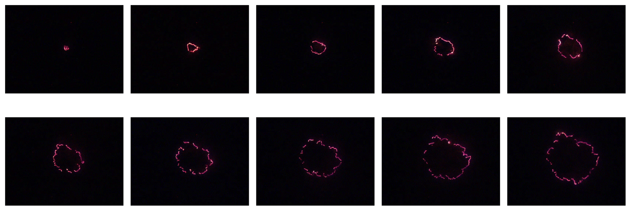
Figure 1A sequence of burn patterns on a sheet of wax paper observed at times of 1, 6, 11, 16, 21, 26, 31, 36, 41, and 46 s for the third microfire. Time increases from left to right, and then down.
The potassium nitrate treatment protocol was adopted for two reasons. First, it prevented flaming and, in fact, induced smouldering combustion. This was important from a lab safety standpoint. Second, flames tend to obscure the pattern of combustion, and this leads to additional image processing issues when extracting the data from the video footage. To further simplify the image processing methodology, these experimental runs were conducted in darkness. This resulted in video footage in which only burning sites were visible; for example, see the screenshots from one of the experimental runs that are displayed in Fig. 1.
A total of 10 microfires were obtained, but only six were retained for further study, due to issues deemed to be unrelated to the study. These issues had to do with difficulties in processing the images from the video streams, due to the presence of fire-spotting, which produced small fires outside the perimeter of the original fire, and due to accidental changes in lighting, which interacted with the reflectivity of the waxed paper. In both cases, this rendered data that will be studied in the future, but which were not amenable to the very quick and simple data extraction and image segmentation procedures that will be described later. In future work, we plan to develop new image segmentation methodology to handle these situations, but as our real focus here is on applying a stochastic model to real data, we feel this is beyond the scope of the current paper.
2.2 Data extraction and segmentation
The open-source program ffmpeg (Libav, 2010–2013) was used to freeze-frame each movie at approximately half-second intervals to obtain clear image captures with timestamps. These captured images were then saved as JPEG files, readable in the R system (R Core Team, 2018). For illustrative purposes, the images for the third experimental run are shown in Fig. 1 (the images for the remaining five microfires can be found in the Supplement submitted along with this paper). The original images were a combination of several colours: yellow, red, grey, black, etc. In order to convert the image matrices into a usable form, conversion to three colours, red (burning), green (fuel), and black (burnt out), was necessary.
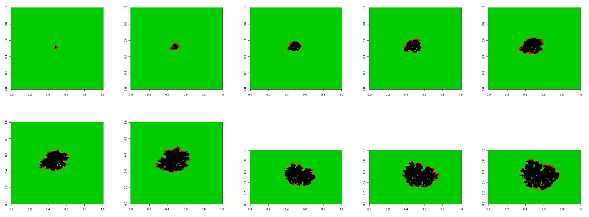
Figure 2Thresholded patterns for the third microfire. Unburned areas are coded as the light grey (green, if in colour), burning regions are at an intermediate grey shade (or red), and burnt regions are black.
This image segmentation problem was greatly simplified because of the use of darkness in the experimental setup. Each grid cell is unburned until it burns (and is lit up in the video footage) and is burnt out for all remaining time. Therefore, the time(s) at which each grid cell burns can be identified from the time series of the red, green, and blue (rgb) measurements. The series corresponding to red is most useful for this purpose. Prior to burning, the values are at or near 0; thus all images corresponding to these times can be set to “green”. After burning, the values are again at or near 0; these can be set to “black”. The values at the time(s) of burning can be set to “red”. The resulting patterns, corresponding to the images in Fig. 1 are displayed in Fig. 2.
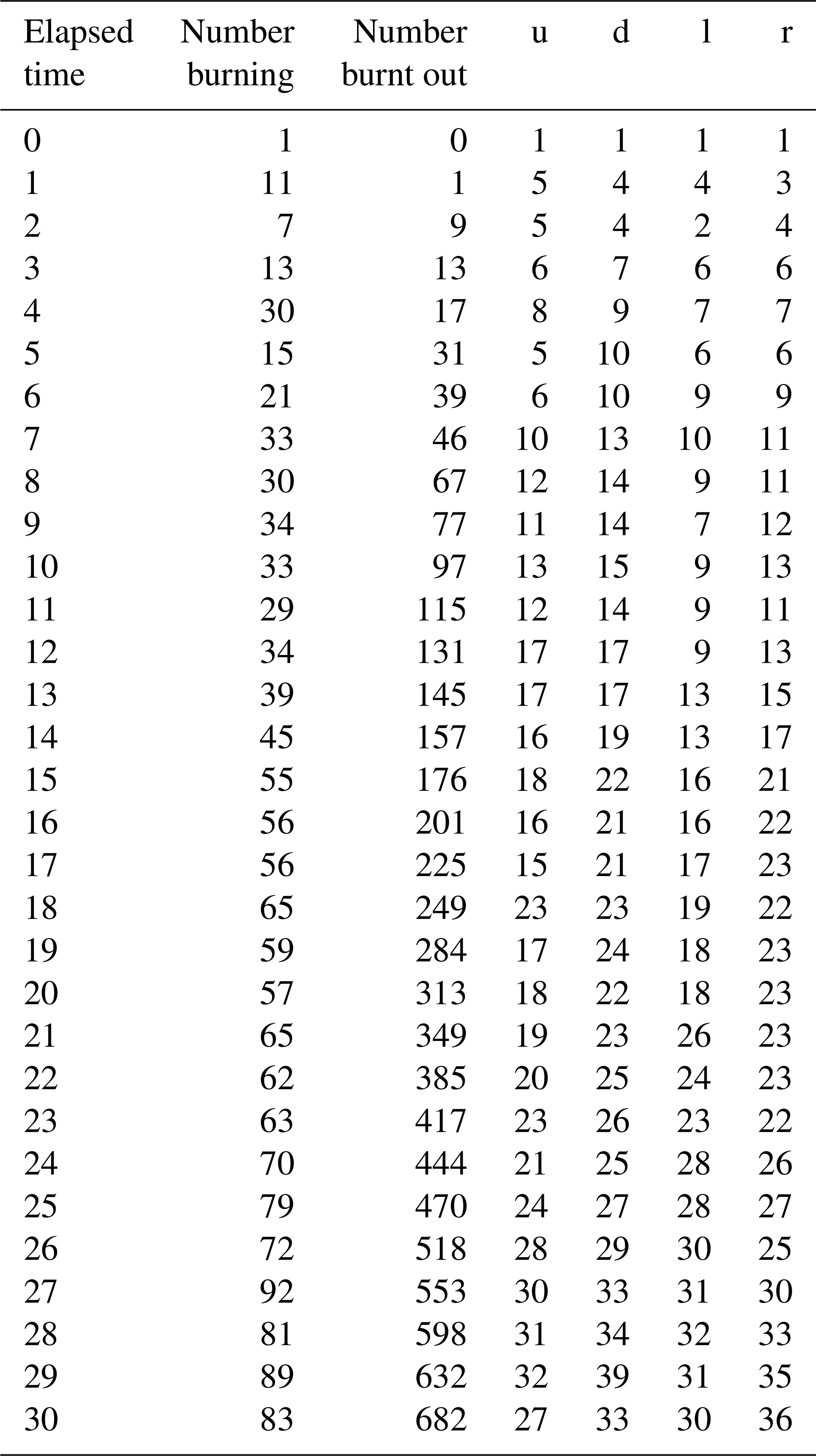
Finally, the colour-coded images were converted to a numeric matrix corresponding to the green, red, and black pixels of the image array. We assigned the colour green to the value 0, red to the value 1, and black to the value 2. The numbers of 0, 1, and 2 were counted, which gave the numbers of unburned fuel sites, the number of burning sites, and the number of burnt-out sites. In addition, the number of fuel sites neighbouring burning sites at each time point were also counted. To illustrate, the counts for each of these statistics during the first 30 s are listed in Table 1 for the third microfire. The detailed smoldering experiment data for all the microfires are provided in the Supplement.
Table 1Counts of the six statistics for the third microfire at a sequence of times (measured in seconds): numbers of burning sites, burnt-out points, and the four nearest-neighbour counts.
We now develop the methodology required to fit the grid-based fire spread model to the data extracted from a sequence of images of a growing fire. Referring to data such as in Table 1, let X(t) denote the number of burning sites at time t and Y(t) denote the number of sites that are burnt out by time t. In addition, let Bℓ(t), Br(t), Bu(t), and Bd(t) denote the number of burning sites with unburnt fuel in the site immediately on their left (west), right (east), above (north/up), or below (south/down), respectively. Also, let
and
According to the model rules and arguing as in Braun and Kulperger (1993), we have the relations
and initial conditions of y(0)=0 and x(0)=1.
These equations hold for both the original Boychuk model as well as the variant introduced by Braun and Woolford (2013). This result seems surprising since the Braun and Woolford variant is non-Markovian, while the Boychuk model is. However, it is important to note that the differential equations are for population level quantities. They are also only a partial description of the process dynamics. However, they contain enough process information to allow for construction of moment estimators for the process parameters as we now demonstrate.
The notation in the ensuing discussion can be simplified by making the substitution
Then
By adding Eqs. (1) and (1), we obtain:
3.1 Moment and continuous least-squares estimation
We can estimate the functions x(t) and y(t) using X(t) and Y(t), respectively. In fact, improved estimates of these functions can be obtained by applying a local linear kernel smoother to the (t,X(t)) data and (t,Y(t)) data respectively. Similarly, estimates of g(t) can be improved by a local constant smoother. We used the locpoly function in the KernSmooth package (Wand, 2015) with an automatically selected smoothing parameter. The software also allows for estimation of the first derivatives x′(t) and y′(t) from the same data sets (see Wand and Jones, 1995, for example).
Substituting these local linear kernel-smoothing-based estimates and into Eq. (1), continuous least squares can then be applied to estimate μ. That is,
where and are the smoothed estimates described in the preceding paragraph.
An estimator for λ can be obtained from the estimated version of Eq. (2) similarly:
3.2 Estimation of scale
It is important to note that the pixel size induced by the camera specifications has nothing to do with the size of the grid cells imposed on the lattice underlying the stochastic spread model. Thus, a scale parameter must be selected, which is used to expand or contract the default pixel sizes so that the spread model process can be used as a realistic approximation for the actual data. Specifically, we adjust the scale factor until the range of the observed data matches the range of the simulated data by using the estimated parameters.
In this paper, slightly different amounts of scaling are used for six replicates of the dark smouldering experiment in order to match the pixel size for the camera and the grid cell size on the lattice. The scale factors for all replicates are listed in Table 2. Note that these scale factors are estimated specifically for our microfire data only. One can reproduce the same results by using this fire spread model, based on the same microfire data.
Table 2Estimates of stochastic spread model parameters, μ and λ, based on data from each of six microfires. The grid cell sizes used in the spread model were taken as the camera pixel size divided by the given scale factor. The two rightmost columns of the table give the medians of the estimates of μ and λ for 100 simulated data sets generated according to the fitted stochastic spread model using the observed-data estimates of μ and λ.
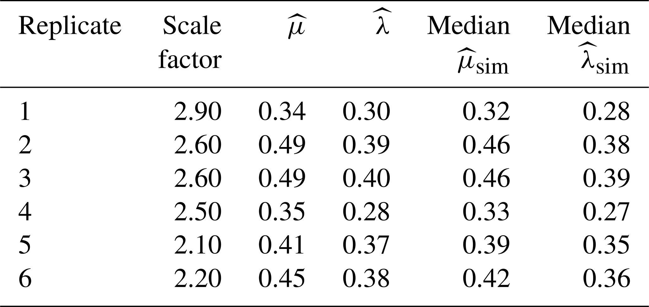
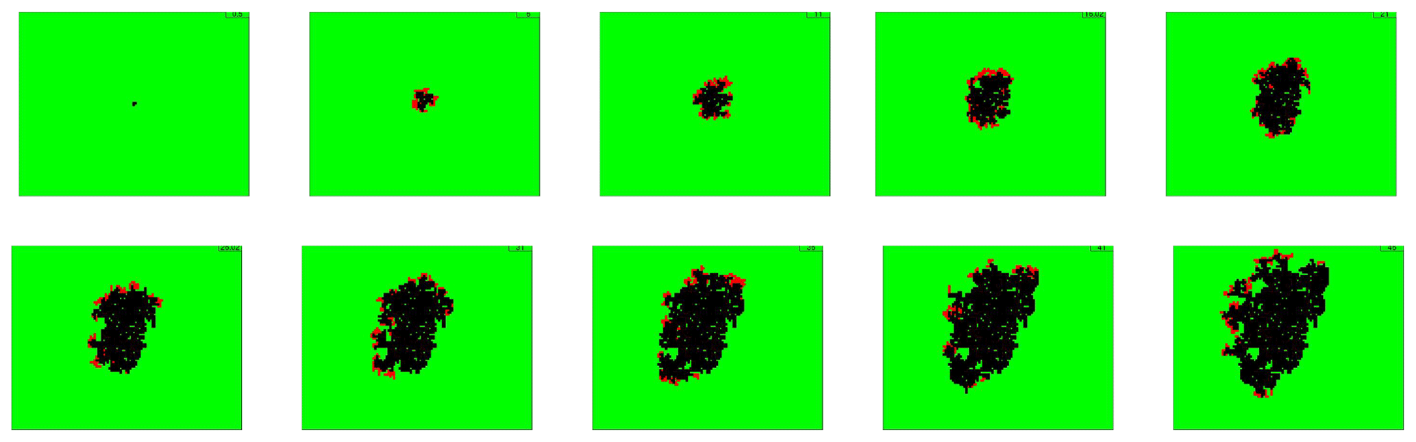
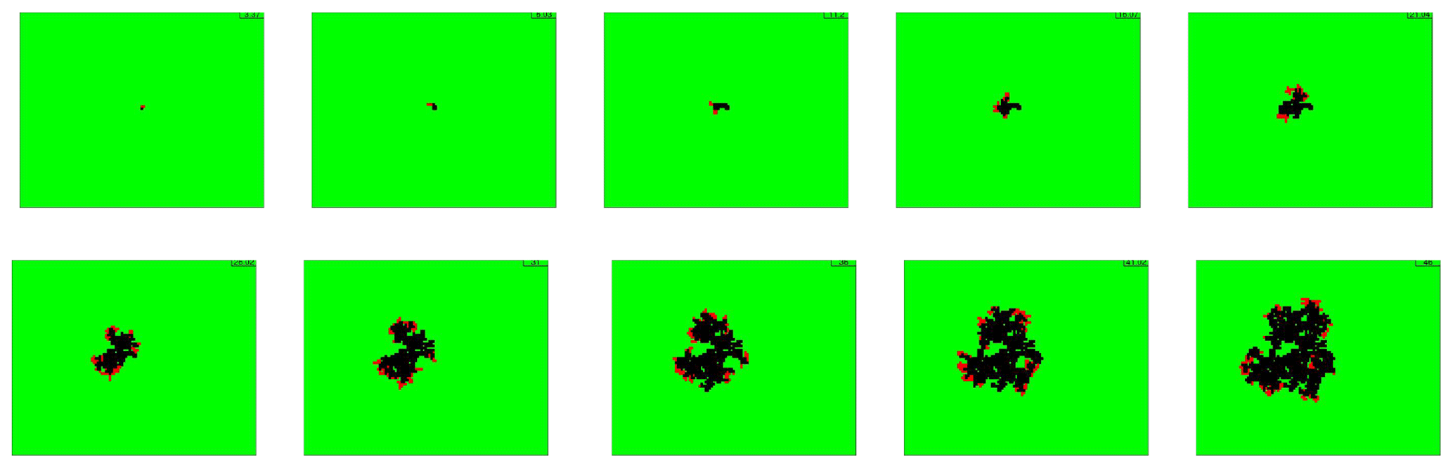
Figure 3A simulation run of the model fit to the observed data from Figs. 1 and 2. Colour coding is the same as described in Fig. 2.
As noted earlier, the sequence of fire images is displayed in Fig. 1 for one of the microfires. The corresponding thresholded images are displayed in Fig. 2. Based on these images, counts of the various statistics (as listed in Sect. 3) were taken, at a number of different grid resolutions (as discussed in Sect. 3.2). Table 1 displays the counts at one of the resolutions, and the third row of Table 2 contains the resulting parameter estimates and the amount of scaling performed to increase the pixel size.
The remaining rows of Table 2 contain the parameter estimates and scalings required for the other five microfires. We see that the fires required different amounts of scaling, and the estimates of μ range from 0.34 grid cells per second to 0.49 grid cells per second. The estimates of λ range from 0.28 to 0.40. In all cases, the burn out parameter exceeds the spread rate parameter, which suggests a subcritical process. Thus, the fires would be expected to ultimately die out with probability 1.
4.1 Parameter estimation bias and variability
By simulating from the fitted model and re-estimating the parameters, it is possible to assess bias and variability of the parameter estimates. We have chosen to display the results of this assessment for the third microfire in Fig. 5 using box plots to graphically summarize the distribution of the estimates μ and λ for the simulated data sets. Horizontal lines have been drawn to indicate the locations of μ (solid) and λ (dashed). What is immediately evident from the graphs is that both μ and λ appear to be underestimated in the simulations: the medians of the estimates from the simulated data are both about 0.02 less than the values used to produce the simulated data.
The box plots also show that the distributions of the parameter estimates are approximately symmetric, and the amount of variability is of the same order as the bias. That is, if these simulations were viewed as a parametric bootstrap, the standard errors for the two estimators are approximately 0.01. Thus, the bias dominates the MSE, and the root-MSE is approximately 0.022 for both estimators.
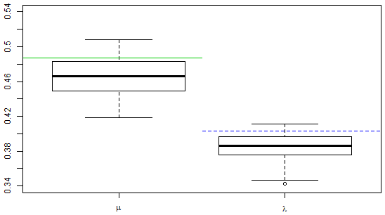
Figure 5Comparisons of parameter estimates between simulations and observed data for the third microfire. The box plots represent samples of estimates based on 100 simulations of the fitted stochastic spread model. The solid horizontal line represents the estimated value of μ and the dashed horizontal line represents the estimate of λ, based on the observed data.
Box plots for the other five fires (not shown) are quite similar to what appears in Fig. 5. All six fires exhibit the same degree and direction of bias. Table 2 contains information on the medians for the estimates of λ and μ from simulations of each of the fitted models. In all cases, the medians of the parameter estimates from the simulated data are slightly below the parameter values used in the simulations.
4.2 Model assessment
To assess the adequacy of the grid-based fire spread model for this particular data set, we again simulated realizations of fire spread at the estimated parameter values, using the chosen grid resolution. The results are the sequence of pictures in Fig. 3. The images have been plotted at approximately 5 s intervals. We see from these pictures that the fire size and the thickness of the fire perimeter are similar to the analogous quantities for the thresholded images at corresponding times. The boundary is somewhat less smooth in the simulation pictures than in the actual fire, but the overall shapes are fairly similar. The simulated fire appears to have grown somewhat larger than the observed fire. However, Fig. 4 shows the results of another simulation run where similar qualitative behaviour is evident but where the fire sizes tend to be somewhat smaller than observed.
Such plots are limited in their usefulness. In this case, we can see that there are differences between the simulated pictures and the actual data, but it is difficult to tell if these differences are due to the variability we are trying to model or if these are failures of the model itself.

Figure 6Comparisons between data from 100 simulation runs and observed data from six microfires. (a) Number of simulated (grey) and observed (blue) burning sites versus time; (b) number of simulated (grey) and observed (blue) burnt-out sites versus time; (c–f) number of simulated (grey) and observed (blue) neighbourhood counts versus time. The black curve in each panel corresponds to the observed data from the third microfire, upon which the estimates of μ and λ underlying the simulated data are based.
As another check on the appropriateness of the model, we can compare the burning cell counts, burnt-out cell counts, and nearest-neighbour statistics for the original data with simulated data from the fitted model (using data from the third microfire only). Figure 6 shows the results of 100 simulated realizations (plotted in grey) with the observed counts for all the other fires (plotted in blue) against time; the observed data for the third microfire are plotted in black.
What is evident from this set of plots is that the range and distribution of simulated counts of burning sites (based on the observed data from one fire) match the observed range and distribution of burning sites for other fires very well. Except for a location shift in the distribution of simulated burnt-out sites and neighbourhood statistics, we also see similarities in the range and distribution in these cases. The location shift is likely due to the estimation bias discussed earlier. Note that by increasing both μ and λ slightly, we will not see much change in the total number of burning sites over time, but we will see many more burnt-out sites, for example. It is also noteworthy that for one of the actual fires, there were instances of flaming which distorted the camera images at two time points, reflected in the anomalous spikes in Fig. 6.
These observations provide strong evidence that the model is doing well at capturing distributional behaviour in these dimensions. Further assessment of model goodness of fit is provided in the Supplement submitted along with this paper.
This work is part of an ongoing investigation into the suitability of a simple grid-based interacting particle system for stochastically modelling forest fire spread. Ultimately, we wish to fit such a model to sequences of satellite-based photographs of wildfires. Then, simulations of the model could be used to produce the maps of fire spread risk that are in demand by forest fire managers. Before this can happen, experiments under other conditions on slope and different kinds of fuel and wind conditions must be carried out. This paper represents the analysis of one such set of experiments, and the results appear promising.
What can be firmly concluded is that the parameters for the simplest case of the model can be estimated from a sequential set of photographs from a fire, using differential equations for the moments of certain statistics derivable from a video clip of a fire. A critical element of this estimation is that of scale. We have shown that the “natural” grid cell size can be determined, at least crudely, from a characteristic of the fire: the ratio of burnt-out area to the square of the burning area. Information about the scale is also likely related to the variability of the fire spread; this is an issue that can be addressed by studying an ensemble of experimental fires conducted under the same conditions. It should be noted that we have thresholded individual images; other methods taking account of the time sequence at each pixel (and at neighbouring pixels) may lead to more accurate counts of neighbourhood statistics and burning and burnt-out sites, given that flames and/or smoke cause distortions. The paper by Fang et al. (2007) indicates another possible approach that could be adopted.
We have developed some goodness-of-fit methods. A simple visual assessment based on comparing burn patterns simulated from the fitted model with the observed pattern is a useful, if limited, first step. This method of assessment gives some assurance that the model appears to reasonably fit the data. However, such a comparison is highly subjective and will not necessarily generalize to cases where, for example, the assumption of isotropy is invalid. The very nature of a stochastic model leads to different possible patterns under the same conditions. Hence, the following question arises: how different can the patterns be from the observed pattern before one might conclude that the model has failed?
What is needed, in general, is a metric for scoring spatial burn pattern maps that evolve over time in terms of their shape and boundary characteristics. In this paper, we have proposed the four nearest-neighbourhood statistics as belonging to such a set of measures. On the basis of an informal bootstrap procedure applied to these statistics, we have a fair degree of confidence that the model is capturing some of the stochastic behaviour of the actual fire.
For the purposes of reproducible research, we have uploaded the data (frozen video frames) and R code to the Open Science Framework repository. See Braun et al. (2018). The frozen video frames can be downloaded and unzipped, and then the file called MainDriver.R can be run in R to process the data as carried out in this paper.
The supplement related to this article is available online at: https://doi.org/10.5194/ascmo-5-57-2019-supplement.
DGW and WJB developed the modelling methodology and under their direction, XJW and JRJT designed and carried out the experiments. XJW and WJB designed and carried out the simulation experiments that were used to assess the model.
The authors declare that they have no conflict of interest.
The authors gratefully acknowledge support from the Natural Sciences and Engineering Research Council of Canada through individual Discovery Grants to W. John Braun and Douglas G. Woolford and the Canadian Statistical Sciences Institute through its Collaborative Research Team funding program. The authors are also grateful to Andrew Jirasek for facilitating access to his laboratory where the experiments were conducted.
This paper was edited by Christopher Paciorek and reviewed by two anonymous referees.
Albert-Green, A., Dean, C. B., Martell, D. L., and Woolford, D. G.: A methodology for investigating trends in changes in the timing of the fire season with applications to lightning-caused forest fires in Alberta and Ontario, Canada, Can. J. Forest Res., 43, 39–45, 2012.
Anderson, K., Reuter, G., and Flannigan, M.: Fire-growth modeling using meteorological data with random and systematic perturbations, Int. J. Wildland Fire, 16, 174–182, 2007.
Boychuk, D., Braun, W. J., Kulperger, R. J., Krougly, Z. L., and Stanford, D. A.: A stochastic model for forest fire growth, INFOR, 45, 9–16, 2007.
Braun, W. J. and Kulperger, R. J.: Differential equations for moments of an Interacting particle process on a lattice, J. Math. Biol., 31, 199–214, 1993.
Braun, W. J. and Woolford, D. G.: Assessing a stochastic fire spread simulator, J. Environ. Inform., 22, 1–12, 2013.
Braun, W. J., Woolford, D. G., and Wang, X.: Microfire modelling, Open Science Framework, July 13, http://osf.io/9b7tp, last access: 13 July 2018.
Fang, Z. Moller, T., Hamarneh, G., and Celler, A.: Visualization and exploration of spatio-temporal medical image data sets, Graph. Inter., 2007, 281–288, 2007.
Finney, M. A.: FARSITE: Fire Area Simulator-model development and evaluation, Res. Pap. RMRS-RP-4, U.S. Department of Agriculture, Forest Service, Rocky Mountain Research Station, Ogden, UT, USA, 2004.
Flannigan, M. D. and Van Wagner, C.: Climate change and wildfire in Canada, Can. J. Forest Res., 21, 66–72, 1991.
Flannigan, M. D., Logan, K. A., Amiro, B. D., Skinner, W. R., and Stocks, B. J.: Future area burned in Canada, Climatic Change, 72, 1–16., https://doi.org/10.1007/s10584-005-5935-y, 2005.
Garcia, T., Braun, W. J., Bryce, R., and Tymstra, C.: Smoothing and bootstrapping the Prometheus Fire Spread Model, Environmetrics, 19, 836–848, 2008.
Gillett, N. P., Weaver, A. J., Zwiers, F. W., and Flannigan, M. D.: Detecting the effect of climate change on Canadian forest fires, Geophys. Res. Lett., 31, L18211, https://doi.org/10.1029/2004GL020876, 2004.
Han, L. S. and Braun, W. J.: Dionysus: A stochastic fire growth scenario generator, Environmetrics, 25, 431–442, 2014.
Libav developers: ffmpeg, version 0.8.10–6:0.8.10-0ubuntu0.13.10.1 [Software], available at: http://ffmpeg.org/ (last access: 30 November 2018), 2000–2013.
Parisien, M. A., Kafka, V. G., Hirsch, K. G., Todd, J. B., Lavoie, S. G., and Maczek, P. D.: Using the Burn-P3 simulation model to map wildfire susceptibility, Natural Resources Canada, Canadian Forest Service, Northern Forestry Centre, Edmonton, AB, Canada, Information Report NOR-X-405, 2005.
R Core Team: R: A language and environment for statistical computing, R Foundation for Statistical Computing, ISBN 3-900051-07-0, Vienna, Austria, available at: https://www.R-project.org/, last access: 15 March 2018.
Taylor, S. W., Woolford, D. G., Dean, C. B., and Martell, D. L.: Wildfire prediction to inform management: statistical science challenges, Stat. Sci., 28, 586–615, 2013.
Tymstra, C.: Prometheus: The Canadian Wildland Fire Growth Model, Forest Protection Division, Alberta Sustainable Resource Development, Edmonton, AB available at: http://www.firegrowthmodel.com (last access: 9 April 2019), 2005.
Wand, M.: KernSmooth: Functions for Kernel Smoothing Supporting Wand & Jones (1995), R package version 2.23-15, available at: https://CRAN.R-project.org/package=KernSmooth (last access: 15 March 2018), 2015.
Wand, M. P. and Jones, M. C.: Kernel Smoothing, Chapman and Hall, London, UK, 1995.
Weber, M. G. and Stocks, B. J.: Forest fires and sustainability in the boreal forests of Canada, Ambio, 27, 545–550, 1998.
Woolford, D. G., Cao, J., Dean, C. B., and Martell, D. L.: Characterizing temporal changes in forest fire ignitions: looking for climate change signals in a region of the Canadian boreal forest, Environmetrics, 21, 789–800, 2010.
Woolford, D. G., Dean, C. B., Martell, D. L., Cao, J., and Wotton, B. M.: Lightning-caused forest fire risk in Northwestern Ontario, Canada, is increasing and associated with anomalies in fire weather, Environmetrics, 25, 406–416, 2014.
Wotton, B. M. and Flannigan, M. D.: Length of the fire season in a changing climate, Forest. Chron., 69, 187–192, 1993.
Wotton, B. M., Nock, C. A., and Flannigan, M. D. : Forest fire occurrence and climate change in Canada, Int. J. Wildland Fire, 19, 253–271, 2010.
Zhang, J., Zhang, Y.-C., Alstrom, P., and Levinsen, M. T.: Modeling forest fire by a paper-burning experiment, a realization of the interface growth mechanism, Physica A, 189, 383–389, 1992.