NWP-based lightning prediction using flexible count data regression

Simon, Thorsten; Mayr, Georg J.; Umlauf, Nikolaus; Zeileis, Achim

doi:https://doi.org/10.5194/ascmo-5-1-2019

Articles | Volume 5, issue 1

https://doi.org/10.5194/ascmo-5-1-2019

Articles | Volume 5, issue 1

04 Feb 2019

| 04 Feb 2019

NWP-based lightning prediction using flexible count data regression

Thorsten Simon, Georg J. Mayr, Nikolaus Umlauf, and Achim Zeileis

Abstract

A method to predict lightning by postprocessing numerical weather prediction (NWP) output is developed for the region of the European Eastern Alps. Cloud-to-ground (CG) flashes – detected by the ground-based Austrian Lightning Detection & Information System (ALDIS) network – are counted on the 18×18 km² grid of the 51-member NWP ensemble of the European Centre for Medium-Range Weather Forecasts (ECMWF). These counts serve as the target quantity in count data regression models for the occurrence of lightning events and flash counts of CG. The probability of lightning occurrence is modelled by a Bernoulli distribution. The flash counts are modelled with a hurdle approach where the Bernoulli distribution is combined with a zero-truncated negative binomial. In the statistical models the parameters of the distributions are described by additive predictors, which are assembled using potentially nonlinear functions of NWP covariates. Measures of location and spread of 100 direct and derived NWP covariates provide a pool of candidates for the nonlinear terms. A combination of stability selection and gradient boosting identifies the nine (three) most influential terms for the parameters of the Bernoulli (zero-truncated negative binomial) distribution, most of which turn out to be associated with either convective available potential energy (CAPE) or convective precipitation. Markov chain Monte Carlo (MCMC) sampling estimates the final model to provide credible inference of effects, scores, and predictions. The selection of terms and MCMC sampling are applied for data of the year 2016, and out-of-sample performance is evaluated for 2017. The occurrence model outperforms a reference climatology – based on 7 years of data – up to a forecast horizon of 5 days. The flash count model is calibrated and also outperforms climatology for exceedance probabilities, quantiles, and full predictive distributions.

Download & links

Article (PDF, 4083 KB)

Download & links

How to cite.

Received: 04 Jul 2018 – Revised: 02 Jan 2019 – Accepted: 08 Jan 2019 – Published: 04 Feb 2019

1 Introduction

Lightning in Alpine regions is associated with events such as convection, thunderstorms, extreme precipitation, high wind gusts, flash floods, and debris flows. In order to predict the probability of lightning events (i.e. thunderstorms), numerical weather prediction (NWP) output is often postprocessed by logistic regression (Schmeits et al., 2008; Gijben et al., 2017; Bates et al., 2018; Simon et al., 2018) in which lightning detection data serve as a proxy for the occurrence of thunderstorms. However, these studies present methods to predict only whether a thunderstorm might take place or not.

The objective of the present work is to extend this approach by modelling the intensity of thunderstorms with a model for the time and space variations of lightning counts. From a statistical perspective this means that not a Bernoulli distribution, which is determined only by the occurrence probability, has to be employed, but a parametric count data distribution. Classically, count data are modelled by a Poisson distribution (Cameron and Trivedi, 2013). However, in practical work data often have excess zeros and/or have a variance larger than their mean, which is called overdispersion¹ in the count data literature (Cameron and Trivedi, 2013).

Figure 1 illustrates such excess zeros and overdispersion. The synoptic weak pressure gradient situation on 18 July 2017 allowed local heating to trigger a number of single-cell storms. Very high lightning flash rate intensities exceeding 40 cloud-to-ground (CG) flashes were observed in 29 boxes (3.2 % of the whole domain) along the main Alpine ridge between 12:00 and 18:00 UTC. However, a large number of boxes (82.2 %) remained devoid of CG lightning.

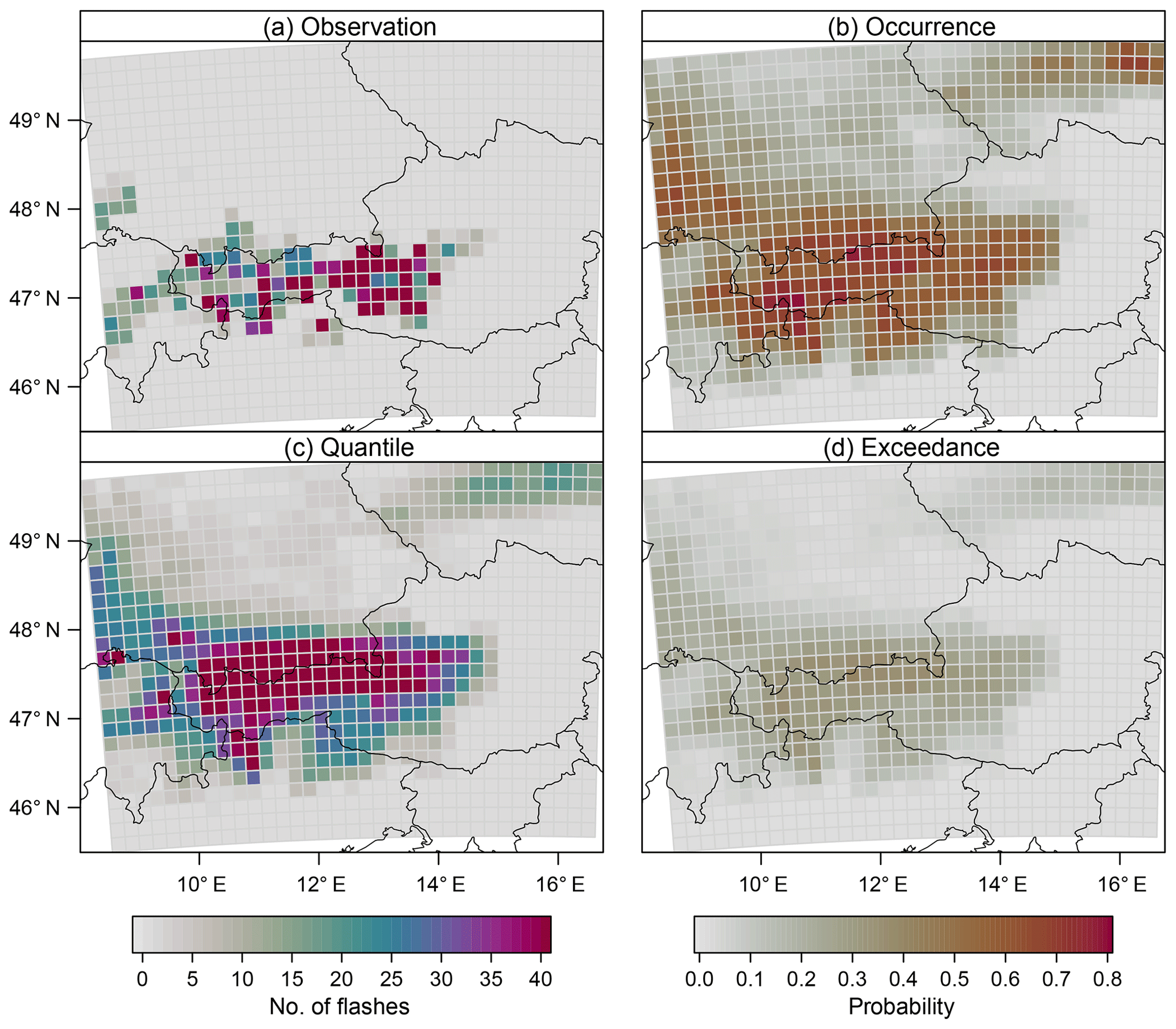
https://www.adv-stat-clim-meteorol-oceanogr.net/5/1/2019/ascmo-5-1-2019-f01

Figure 1A sample prediction case (18 July 2017) for the lightning count model with a lead time of 1 day. (a) Number of observed flashes from 12:00 to 18:00 UTC in a 18×18 km² grid box. (b) Predicted probabilities for the occurrence of lightning events (no. of flashes >0). (c) Predicted 90 % quantiles. (d) Predicted probabilities for exceeding a threshold of 10 flashes in a grid box.

Download

Overdispersed data can be handled by applying a negative binomial distribution (Cameron and Trivedi, 2013). Excess zeros can be accounted for by splitting the distribution into a binary hurdle and a part for positive counts (Mullahy, 1986). The hurdle can be modelled e.g. by logistic regression and the positive counts by a zero-truncated version of the Poisson or negative binomial distribution. Another benefit of the hurdle approach is that the binary hurdle part can serve as a stand-alone model for the occurrence of thunderstorms. Thus, the predictions resulting from the binary hurdle part can be compared directly to the outcome of previous studies that focus on binary response variables (e.g. Schmeits et al., 2008; Simon et al., 2018). The combined model predicts a full probability distribution of lightning counts, which allows one to derive various quantities such as probabilities for the occurrence of thunderstorms and also quantiles and the exceedance of predefined lightning count thresholds (Fig. 1).

Input variables for the statistical models come from a physically based NWP model and capture convection only incompletely. Convection permitting or resolving models with horizontal meshes of 1–3 km are capable of reproducing bulk properties of heat and water vapour (Langhans et al., 2012). In contrast, global NWP systems with a coarser resolution simulate convection with parametric submodels, which may be perturbed stochastically (Buizza et al., 1999). By generating ensembles of a numerical forecast one aims at accounting for uncertainties of small-scale events such as convection.

In this study a set of direct and derived NWP variables from the (global) ECMWF ensemble is employed as covariates for a statistical lightning prediction model. Many different output variables of an NWP ensemble system are potentially good candidates for lightning prediction, e.g. convective available potential energy (CAPE) or convective precipitation. However, next to these potential good candidates any additional variable could improve the prediction even by a small contribution. Moreover, the effect of individual variables might act nonlinearly on the target quantity (lightning counts).

In order to account for nonlinear dependencies we employ additive predictors linked to the parameters of the hurdle model. Each additive predictor potentially consists of several nonlinear terms which are summed up. This statistical framework is often referred to as distributional regression (Fahrmeir et al., 2013; Klein et al., 2015; Wood, 2017) or generalized additive models for location, scale and shape (Rigby and Stasinopoulos, 2005; Umlauf et al., 2018). The selection of a sparse sufficient set of nonlinear terms from the numerous covariates provided by the NWP ensemble is performed using gradient boosting with stability selection. This concept has been used successfully in several studies (e.g. Simon et al., 2018; Thomas et al., 2018).

The final model resulting from the selection procedure is still complex. Different approaches for identifying the nonlinear terms have been proposed, such as penalized maximum likelihood (Wood, 2017), gradient boosting (Mayr et al., 2012), or Markov chain Monte Carlo (MCMC) sampling based on a Bayesian formulation of the problem (Brezger and Lang, 2006). In this study we follow the Bayesian approach, which ensures stable estimation and valid credible intervals for the regression coefficients of our complex model of the present count data distribution (Klein et al., 2015). The MCMC samples allow inferential conclusions to be drawn about the effects and the predictive performance.

Our statistical approach to modelling flash counts (Sect. 2.1) by postprocessing numerical weather prediction output (Sect. 2.2) can be summarized as follows: a parametric distribution for the count data is specified, in which the parameters are linked to additive predictors that contain potentially nonlinear functions of the covariates (Sect. 3.1). Stability selection combined with gradient boosting selects the most influential terms (Sect. 3.2). The selected model is estimated using MCMC sampling (Sect. 3.3), which allows one to draw inferential conclusions about nonlinear terms and out-of-sample predictions (Sect. 4). Finally, in Sect. 5, we build a connection to previous studies, discuss the transferability of the method, and summarize the study.

2 Data

This section describes the lightning detection data (Sect. 2.1) and the numerical weather prediction ensemble data (Sect. 2.2). The data are collected for the region of the European Eastern Alps (Fig. 2), which is exposed to thunderstorms and severe lightning events during summer (Schulz et al., 2005; Simon et al., 2017).

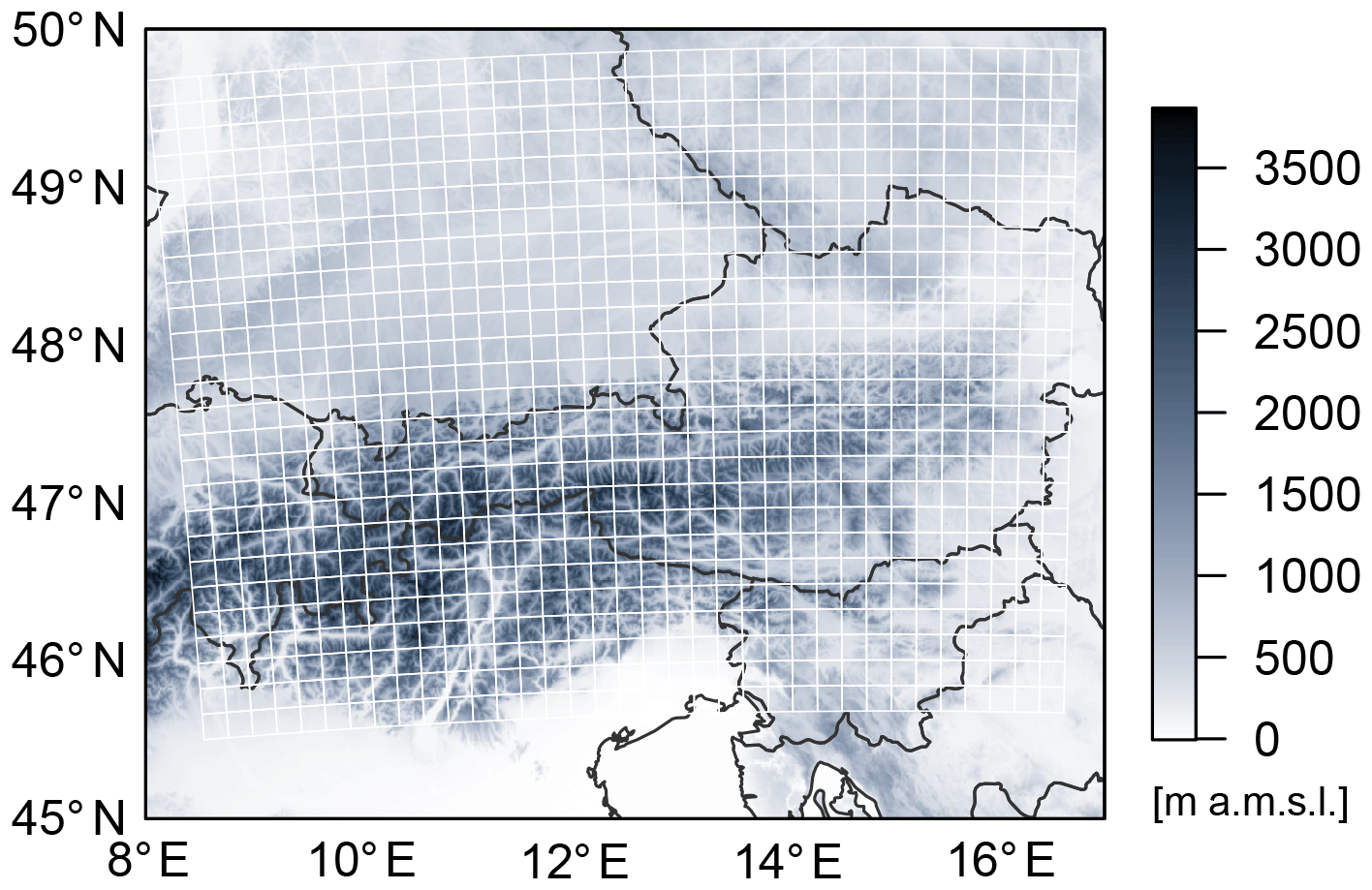
https://www.adv-stat-clim-meteorol-oceanogr.net/5/1/2019/ascmo-5-1-2019-f02

Figure 2Topography of the European Eastern Alps (from SRTM, Farr et al., 2007). Lightning flashes are counted in white grid boxes of 18×18 km².

Download

2.1 Lightning detection data

Lighting data are from the Austrian Lightning Detection & Information System (ALDIS) network (Schulz et al., 2005), for the summer months May–August of the period 2010–2017. The raw ALDIS data are aggregated on a 18×18 km² grid for afternoons (12:00–18:00 UTC). One count refers to one cloud-to-ground flash, which might contain several strokes. We focus on CG flashes, as clustering of CG strokes to an associated flash is more robust than for IC strokes.

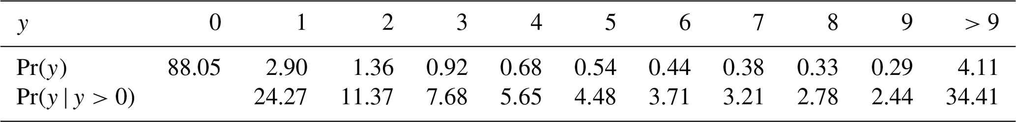
The gridded lightning counts aggregated on this scale during MJJA contain a large amount of zeros (88.05 %). Of the 11.95 % active grid boxes roughly a quarter (24.27 %) contain only a single flash, while approximately a third (34.41 %) contain 10 or more flashes (Table 1). The sample mean and the sample variance of the full data are 1.8 and 136.3, respectively – and 15.05 and 941.06 when calculated over the positive counts, i.e. boxes in which lightning occurred. Thus, the data are heavily skewed with the variance much larger than the mean, which is called overdispersion in the count data literature (Cameron and Trivedi, 2013).

Table 1Unconditional and conditional (given positive counts) probabilities (%) of 18×18 km² grid boxes for the counts of lightning flashes $y = 0, \dots, 9$ .

Download Print Version | Download XLSX

For the given aggregation scale the region (Fig. 2) is described by 910 grid boxes. The season from May to August consists of 123 days, which leads to a sample size of $910 \times 123 = 111 930$ for each year.

2.2 Numerical weather prediction data

Covariates are derived from the ensemble prediction system of the European Centre for Medium-Range Weather Forecasts (ECMWF ENS). Since March 2016 the ECMWF ENS has had a horizontal grid size of approximately 18 km. The temporal resolution of the data is 3-hourly. The summers of 2016 and 2017 serve as the training and evaluation periods, respectively. Moreover, five forecast horizons are considered, where day 1 refers to lead times of 12–18 h of the ensemble initialized at 00:00 UTC. Analogously, day 2, day 3, day 4, and day 5 refer to lead times of 36–42, 60–66, 84–90, and 108–114 h, respectively. All model variables are interpolated bilinearly to the same grid as the lightning data (Fig. 2).

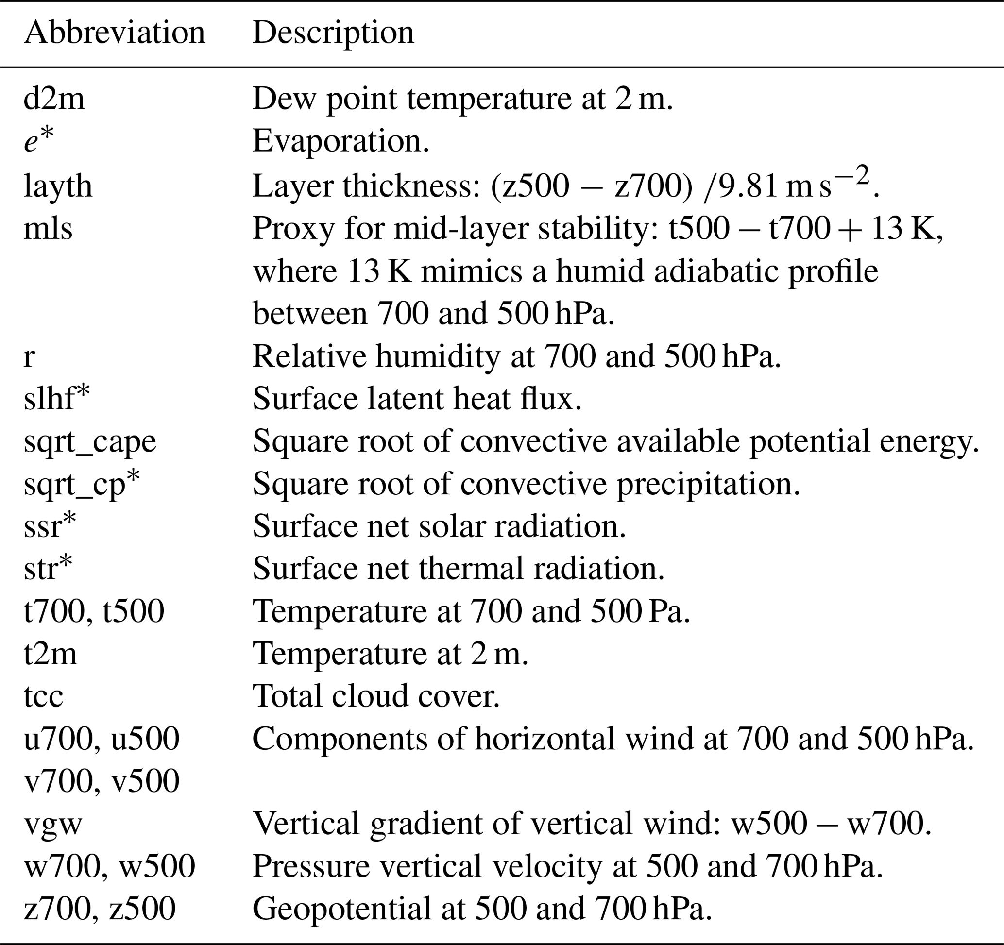
Additional variables are derived by computing vertical differences – i.e. a proxy for mid-layer stability, the layer thickness between 700 and 500 hPa, and the difference of vertical wind for the same two pressure levels. Furthermore we took the square root of highly skewed variables such as convective precipitation and convective available potential energy (CAPE) in order to reduce skewness before employing the statistical model. A full list of direct and derived variables is given in Table 2. Although these variables already cover a wide range of atmospheric processes, the list could still be extended, which will be discussed at the end of this paper.

Table 2An overview of the base covariates from the ECMWF-EPS forecast. The asterisk (^*) indicates accumulated variables. Covariates derived from this base set are discussed in the data section (Sect. 2).

Download Print Version | Download XLSX

For all variables, except for the accumulated fields, the temporal mean over the afternoon, the difference between the values for 18:00 and 12:00 UTC, and anomalies of the three afternoon values from the temporal mean are computed.

Finally, two statistics are computed over the ensemble space, namely the median and the interquartile range (IQR) as measures for location and spread, respectively, of the covariates over the ensemble.

Hereafter the notation of the covariates is as follows. For accumulated fields the name of the variable as listed in Table 2 and its applied statistic over the ensemble are separated by a period. For all other variables the computation applied over the time dimension (mean, difference, or anomaly) is placed in the middle and separated by periods. For instance, to derive t2m.12.median the 2 m temperature is averaged over 12:00, 15:00, and 18:00 UTC for each member of the ECMWF ensemble. This average is subtracted for the value at 12:00 UTC to compute the anomaly. Finally, the median over all 12:00 UTC anomalies is computed over the ensemble space.

3 Methods

This section establishes a statistical count data model for lightning prediction based on NWP outputs from the ECMWF ensemble. The building blocks of this distributional regression model (Fahrmeir et al., 2013; Klein et al., 2015; Wood, 2017; Umlauf et al., 2018) are as follows.

Covariates: direct and derived variables from the NWP data (Sect. 2.2).
Terms: linear or smooth nonlinear functions or interaction surfaces based on the covariates.
Additive predictors: sum of one or more terms to be used for prediction of a distribution parameter.
Probability distribution: a parametric distribution for the lightning counts whose parameters are linked to the additive predictors above.

As the resulting model can become quite complex, especially if all available covariates were considered simultaneously, it is vital to use some form of regularized estimation of the model along with a selection of the relevant terms or covariates. Here, gradient boosting in combination with stability selection is employed for objectively selecting the most influential terms of the additive predictors (Sect. 3.2). The functional forms of the terms selected for the final model are estimated using Markov chain Monte Carlo sampling (Sect. 3.3), which also allows one to draw inferential conclusions about the nonlinear terms and verification scores.

A similar synthesis of methods has been applied previously in Simon et al. (2018) to predict the occurrence probability of thunderstorms, i.e. using only a single additive predictor. Here, a novel extension is presented to a count data distribution with three model parameters and thus three additive predictors. Specifically, a two-part hurdle model is considered (Sect. 3.1) that combines the following components.

Binary hurdle for the occurrence probability, thus addressing the large amount of zeros in the data (i.e. boxes without lightning).
Truncated counts for the distribution of lightning counts (given that lightning occurs) comprising a location parameter and a dispersion parameter to account for the strong overdisperion in the lightning data.

3.1 Count data regression

To account for the large amount of zeros and the strong overdispersion present in the lightning counts $y \in {0, 1, 2, \dots}$ , a hurdle model (Mullahy, 1986) is employed. The hurdle model consists of two parts: one part explicitly models the probability of the occurrence of lightning events; i.e. at least one lightning flash is observed with a grid box. The second part models the number of flashes given that a lightning event takes place.

Hereafter, the two parts of the hurdle model are denoted as binary hurdle part and truncated count part. A Bernoulli distribution for the probability π of lightning (non-zero) events constitutes the binary hurdle part. The actual counts are modelled using a zero-truncated negative binomial distribution, which handles overdispersion and is determined by two parameters for location μ>0 and dispersion θ>0. The zero-truncated negative binomial builds on the negative binomial with the probability mass at zero redistributed towards positive counts (cf. Appendix A).

The hurdle model has the density

\begin{matrix} (1) & f (y | π, μ, θ) = \{\begin{cases} 1 - π & y = 0 \\ π \cdot f_{ZTNB} (y | μ, θ) & y \in {1, 2, \dots}, \end{cases} \end{matrix}

where f_ZTNB is the density of the zero-truncated negative binomial.

When taking the logarithm of Eq. (1) to obtain the associated log-likelihood, a sum emerges where the first summand depends solely on π, i.e. the binary hurdle part, and the second summand depends on μ and θ, i.e. the truncated count part (cf. Appendix A). As a consequence the two parts of the hurdle model can be maximized independently, i.e. with separate estimation, term selection, and prediction.

For the binary hurdle part the probability π for non-zero events is conditioned on (NWP) covariates by an additive predictor η_π,

\begin{array}{l} logit (π) = η_{π} = \underset{baseline climatology}{\underset{︸}{β_{0, π} + f_{1, π} (doy) + f_{2, π} (lon, lat)}} \\ (2) & + f_{3, π} (x_{3}) + \dots + f_{p, π} (x_{p}), \end{array}

where the logit function maps the probability π to the real line. Within the additive predictor, on the right-hand side of Eq. (2), $f_{⋆} (\cdot)$ are functions that are modelled by P-splines in order to account for potentially nonlinear relationships between the response and the covariates doy, lon, lat, and x_j (Wood, 2017). f₁(doy) accounts for an annual cycle, where the day of the year doy serves as a covariate. f₂(lon, lat) is a spatial effect depending on geographical location, i.e. longitude lon and latitude lat. The covariates $x_{3}, \dots, x_{p}$ are the direct and derived parameters from the ECMWF ensemble (Sect. 2.2).

Not all functions $f_{1}, \dots, f_{p}$ are included in the final model, but the relevant terms are selected using gradient boosting combined with stability selection (Sect. 3.2). The resulting final model is estimated using Markov chain Monte Carlo sampling (Sect. 3.3).

For the truncated count part the parameters μ and θ are linked to covariates by additive predictors analogously to the right-hand side of Eq. (2). To ensure positive values for μ and θ, the logarithm serves as a link function:

\begin{array}{l} \log (μ) & = η_{μ} = \underset{baseline climatology}{\underset{︸}{β_{0, μ} + f_{1, μ} (doy) + f_{2, μ} (lon, lat)}} \\ (3) & + f_{3, μ} (x_{3}) + \dots + f_{p, μ} (x_{p}), \\ \log (θ) & = η_{θ} = \underset{baseline  climatology}{\underset{︸}{β_{0, θ} + f_{1, θ} (doy) + f_{2, θ} (lon, lat)}} \\ (4) & + f_{3, θ} (x_{3}) + \dots + f_{p, θ} (x_{p}) . \end{array}

The two additive predictors for log (μ) and log (θ) can encompass different nonlinear terms. The selection of terms is conducted in a joint gradient boosting algorithm, which either selects a term to log (μ) or log (θ) in each iteration (Sect. 3.2).

3.2 Stability selection with gradient boosting

The selection of the most important nonlinear terms within the predictors associated with the parameters π, μ, and θ is performed using gradient boosting combined with stability selection. Gradient boosting is an iterative gradient descent algorithm, where the term which minimizes the residual sum of squares when fitted to the gradient of the log-likelihood is slightly updated in each iteration. The estimates converge to the maximum likelihood estimates when the number of iterations approaches infinity. Early stopping of the iterations ends in regularized estimates of the terms, and also serves as a selection procedure when individual terms are equal to 0 at the final iteration.

The selection of terms for logit(π) (binary hurdle part), and for log (μ) and log (θ) (truncated count part), is performed separately. Hence the binary hurdle part is determined by exactly one parameter (π); the additive predictor for logit(π) is updated in each iteration. Within the truncated count part, which is determined by two parameters (μ and θ), either the additive predictor of log (μ) or log (θ) is updated in each iteration, depending on which update contributes more to the log-likelihood. This updating scheme, called noncyclic in the boosting literature (Mayr et al., 2012), is presented in Appendix B.

If gradient boosting is applied as a stand-alone method the number of iterations – and thus the degree of regularization – can be determined by means of information criteria or cross-validation. Here the main purpose of gradient boosting is to select important terms f_j. It is desirable to avoid the selection of numerous non-informative terms. Stability selection is a convenient resampling method for controlling the number of selected non-informative terms by gradient boosting (Meinshausen and Bühlmann, 2010; Hofner et al., 2015).

Rather than applying the boosting algorithm to all observations, stability selection is based on drawing a subsample half the size of the training data, running the boosting algorithm until a predefined number of terms – 12 and 8 for the binary hurdle and the truncated counts, respectively – is selected. This procedure is repeated many times. Afterwards the relative selection frequencies per nonlinear term are computed. Finally, the terms which were selected in more than, say, 90 % of such subsamples are included in the final model (cf. the algorithm in Hofner et al., 2015). The number of terms being selected before stopping the boosting algorithm and the cut-off selection frequency are chosen in order to establish an upper bound of unity for falsely selected terms (Hofner et al., 2015; Simon et al., 2018).

3.3 Markov chain Monte Carlo sampling

The final model is of a complex form as it contains several nonlinear terms, and thus determining confidence intervals based on asymptotic assumptions might fail. Markov chain Monte Carlo (MCMC) sampling offers an attractive tool to provide valid credible intervals.

To be able to apply this technique to models with additive predictors, the posterior distribution has to be formulated (Brezger and Lang, 2006). The potentially nonlinear functions $f_{*} (\cdot)$ in Eqs. (2), (3) and (4) are modelled by P-spline basis functions (Wood, 2017), which transfers the nonlinear function to a linear regression problem. A multivariate normal distribution serves as prior for the coefficients associated with one function, where the variances of the multivariate normal distributions account for the degree of regularization, which is equivalent to the inverse smoothing parameter in the frequentist approach. Inverse gamma distributions serve as prior densities for these variances. Thus, within the Bayesian framework the degree of regularization is estimated simultaneously during MCMC sampling (Umlauf et al., 2018).

MCMC samples of the posterior distribution can be efficiently generated by approximating a full-conditional distribution using a second order Taylor series expansion of the log-posterior centred at the last state (Gamerman, 1997; Fahrmeir et al., 2013; Umlauf et al., 2018). Moreover, in most situations the structure of the sampling scheme reduces to an iteratively weighted least squares (IWLS) updating step for which highly efficient algorithms are available (Lang et al., 2014).

The statistical models encompassing ECMWF covariates, selected by gradient boosting with stability selection, and the climatological baseline models are estimated by MCMC sampling; 1000 independent realizations of the regression coefficients are drawn from the Markov chains, which enables inference of the effects, predictions, and out-of-sample scores.

4 Results

In this section we present the results of the selection procedure of nonlinear terms for both the binary hurdle part and the truncated count part. Afterwards, we evaluate the performance of the binary hurdle part as an separate model for the occurrence of lightning events, and the combined hurdle model (Eq. 1) as a model for the intensity of lightning events.

4.1 Model selection

4.1.1 Binary hurdle part

The selection of nonlinear terms for the binary hurdle part, i.e. the additive predictor for π, for a lead time of 1 day is visualized in Fig. 3. The gradient boosting algorithm is applied to 100 distinct random subsamples, each half the size of the whole training data until 12 terms are selected. The bars in Fig. 3 indicate the relative frequencies for the terms being selected in the 100 boosting runs.

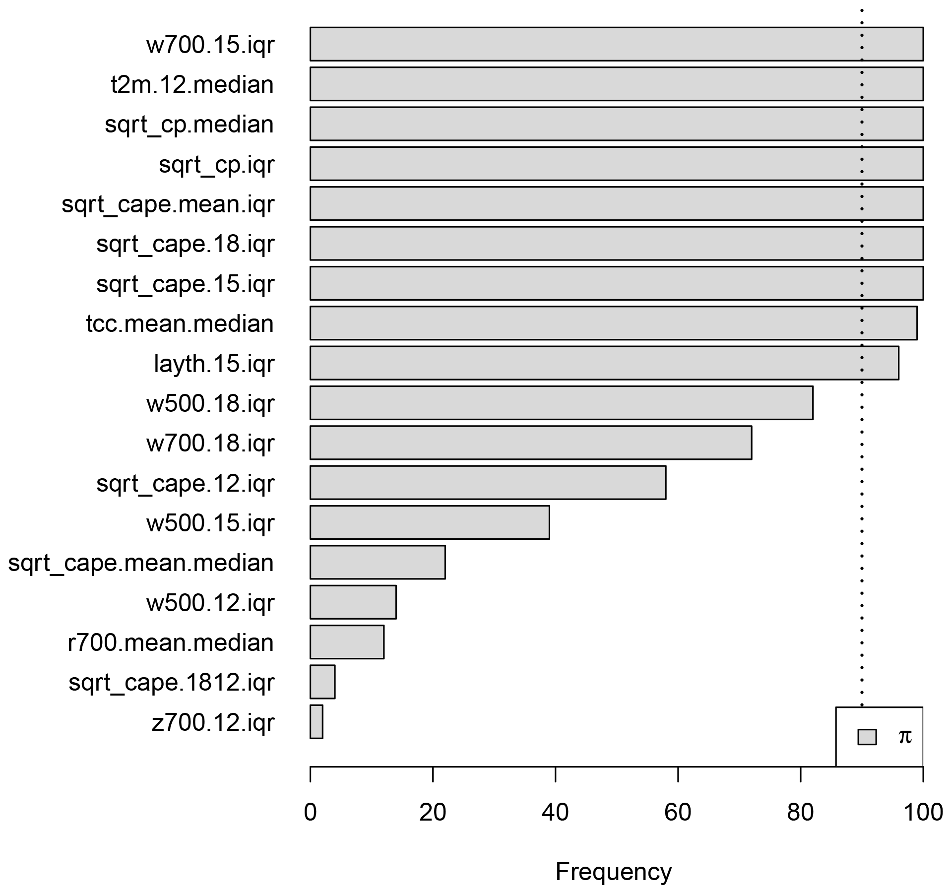
https://www.adv-stat-clim-meteorol-oceanogr.net/5/1/2019/ascmo-5-1-2019-f03

Figure 3Results of the stability selection procedure for the binary hurdle part of the hurdle model for day 1. The variable names on the y axis serve as a placeholder for the associated nonlinear effect. The vertical dotted line marks the threshold of 90 % above which terms are added to the final model.

Download

Nine terms are selected in this case, five of which can be associated either with convective precipitation (cp) or convective available potential energy (cape). Neither the seasonal term f₁(doy) nor the spatial term f₂(lon,lat) is selected, which indicates that temporal and spatial variability is well explained by effects depending only on the ECMWF ensemble covariates.

The selected effects build the (reduced) additive predictor in Eq. (2); 1000 samples of the coefficients for this final model are drawn using MCMC sampling (Sect. 3.3). The mean effects and associated credible intervals (Fig. 4) are computed from these samples. All effects show a smooth and most a monotonic behaviour. The effect of the median of the square root of convective precipitation (sqrt_cp.median) is close to linearity (Fig. 4d).

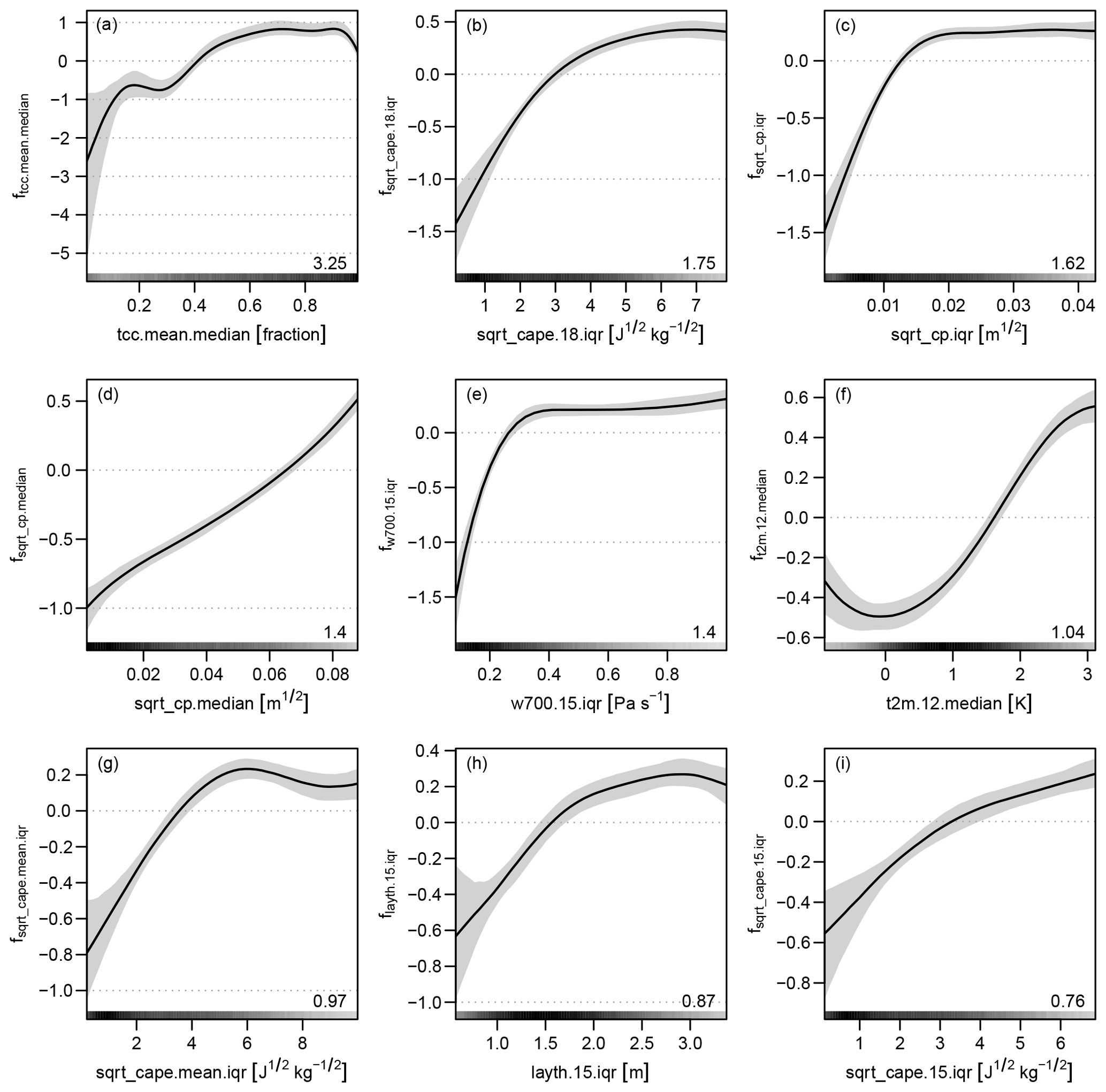
https://www.adv-stat-clim-meteorol-oceanogr.net/5/1/2019/ascmo-5-1-2019-f04

Figure 4Effects and 95 % credible intervals of the occurrence model for day 1 fitted using MCMC sampling. The effects are displayed on the logit scale. The number in the bottom right corner of each panel gives the absolute range of the effect, i.e. the difference between the maximum and the minimum. The shading at the bottom of each panel indicates the density distribution of the corresponding covariate. The x axes are cropped at the 1 % and 99 % percentiles of the respective covariate to enhance graphical representation.

Download

The IQR ensemble statistic appears more often than the median statistic. All the terms associated with the IQR first increase and flatten after some point (Fig. 4b, c, e, g, h, i). Thus, a larger spread of variables such as convective precipitation, CAPE, vertical velocity and layer thickness in the ensemble favours the occurrence of lightning. One meteorological interpretation of this result is that when the synoptic situation does not preclude convection, thunderstorms occur in some of the NWP ensemble members but at different times during the 12:00–18:00 UTC period, which increases the spread of variables in the ensemble.

4.1.2 Truncated count part

The count data part of the hurdle model takes only grid boxes with values greater than zero. Thus the sample size of the training data decreases from 111 930 to 14 099. On this subset of the data the stability selection with gradient boosting is applied in order to find the most relevant effects for the additive predictors of the parameters μ and θ (Eqs. 3 and 4) of the zero-truncated negative binomial. The gradient boosting was run 100 times, each time until eight terms were selected. The result of this procedure is shown in Fig. 5 for the truncated count part with a forecast horizon of 1 day. Three terms are selected for the parameter μ, which is the expectation of the underlying negative binomial distribution, and none for the dispersion parameter θ. Thus, only an intercept β₀ is estimated within the final model of log (θ).

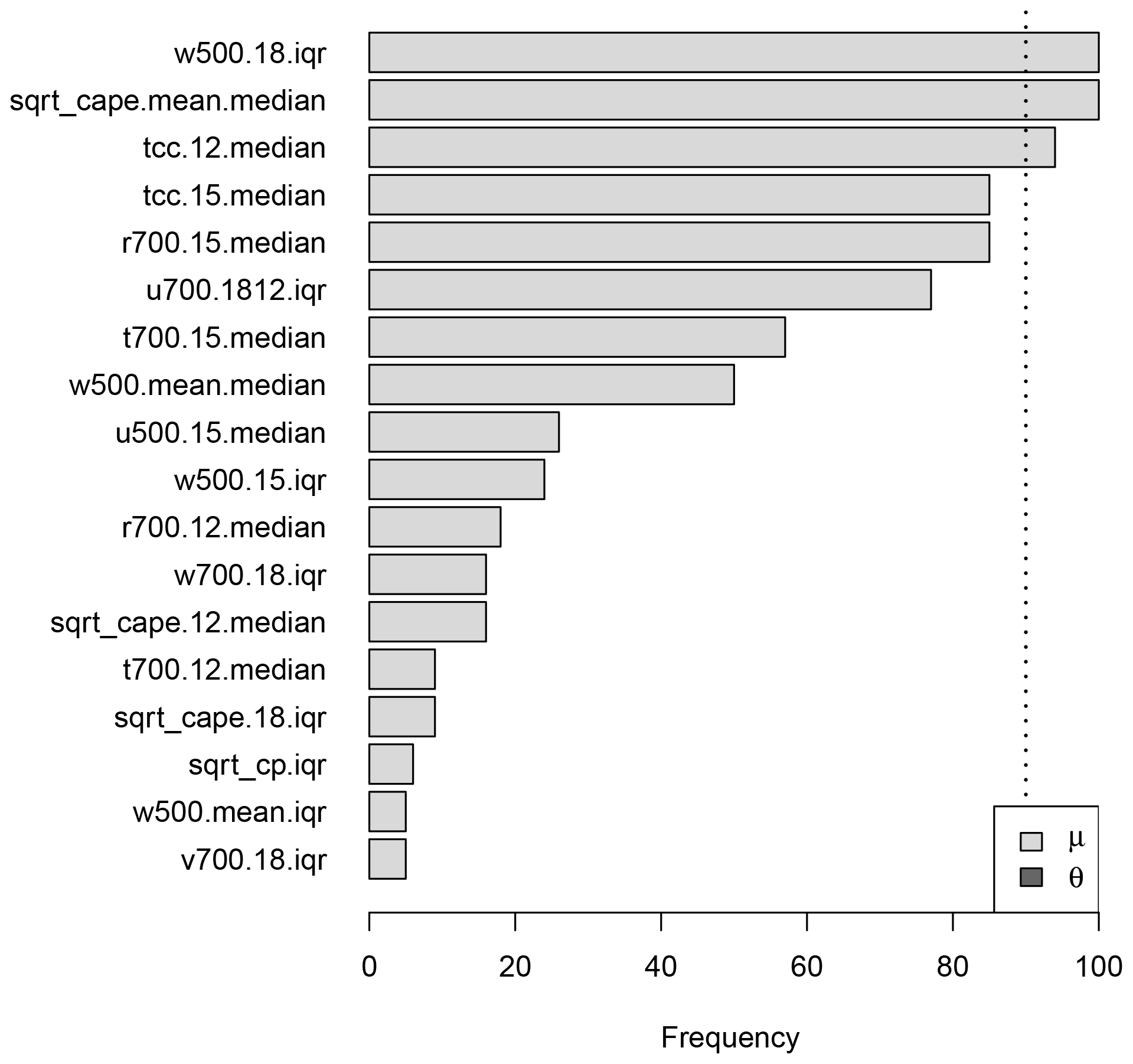
https://www.adv-stat-clim-meteorol-oceanogr.net/5/1/2019/ascmo-5-1-2019-f05

Figure 5As Fig. 3 but for the truncated count part of the hurdle model for day 1. The grey value indicates whether the term is assigned to the predictor of μ or θ. (Note: in this case no terms are selected for the predictor of θ.)

Download

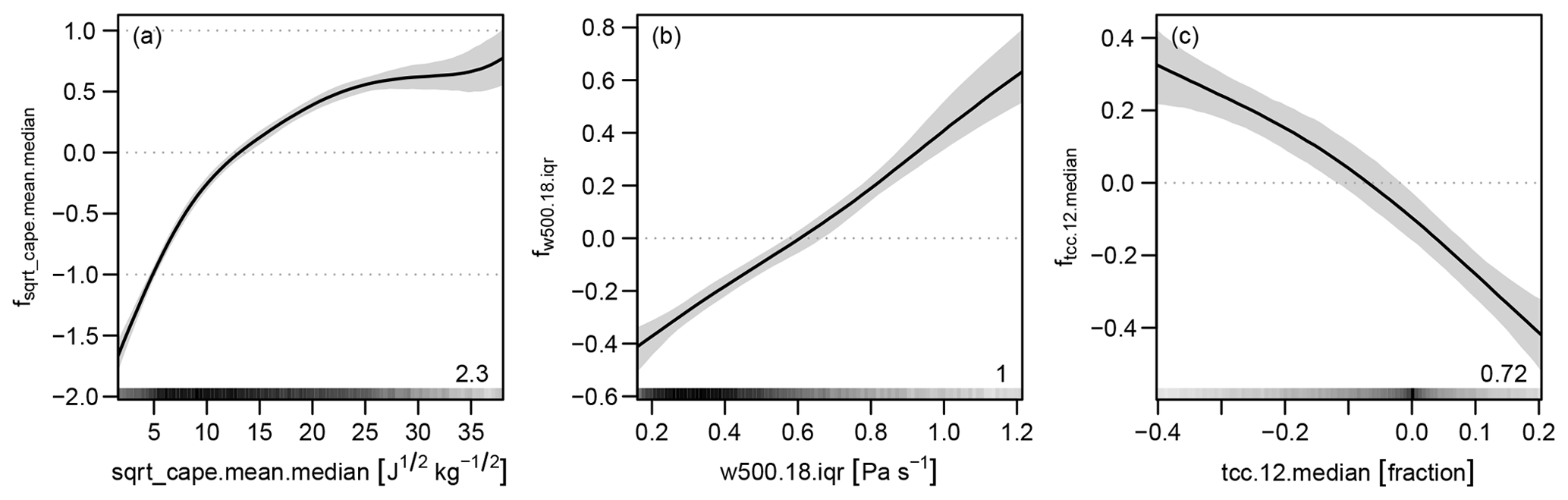
The estimated effects from the MCMC sampling are presented in Fig. 6 on the log scale. The effect with the largest range is the median (over the ensemble) of the mean (over the afternoon) of the square root of cape, which increases monotonically but nonlinearly. The spread (IQR over the ensemble) of the 18:00 UTC anomaly of the vertical velocity at 500 hPa (w500) is associated with a nearly linear effect and its larger spread leads to a larger μ. The median of the 12:00 UTC anomaly of total cloud cover (tcc) reveals a nearly linear effect with a negative slope. The estimated value for θ is 0.199 (0.179, 0.220), which reflects the strong overdispersion of the data.

https://www.adv-stat-clim-meteorol-oceanogr.net/5/1/2019/ascmo-5-1-2019-f06

Figure 6As Fig. 4 but for the intensity model for day 1. All effects are assigned to the predictor of μ and are displayed on the log scale.

Download

4.2 Performance

4.2.1 Occurrence of lightning events

For the evaluation of the predictive performance for the occurrence of lightning events only the probability π is considered. The models with ECMWF ensemble covariates have been estimated on data from 2016 and the data from 2017 are used for an out-of-sample assessment of the performance of the models. The predictions are compared against a climatology, which accounts for seasonal and spatial variations by nonlinear terms (Eq. 2) and is estimated with data from 2010 to 2016. First we present the global scores – averaged over all grid boxes – and afterwards the spatial distribution of skill is analysed.

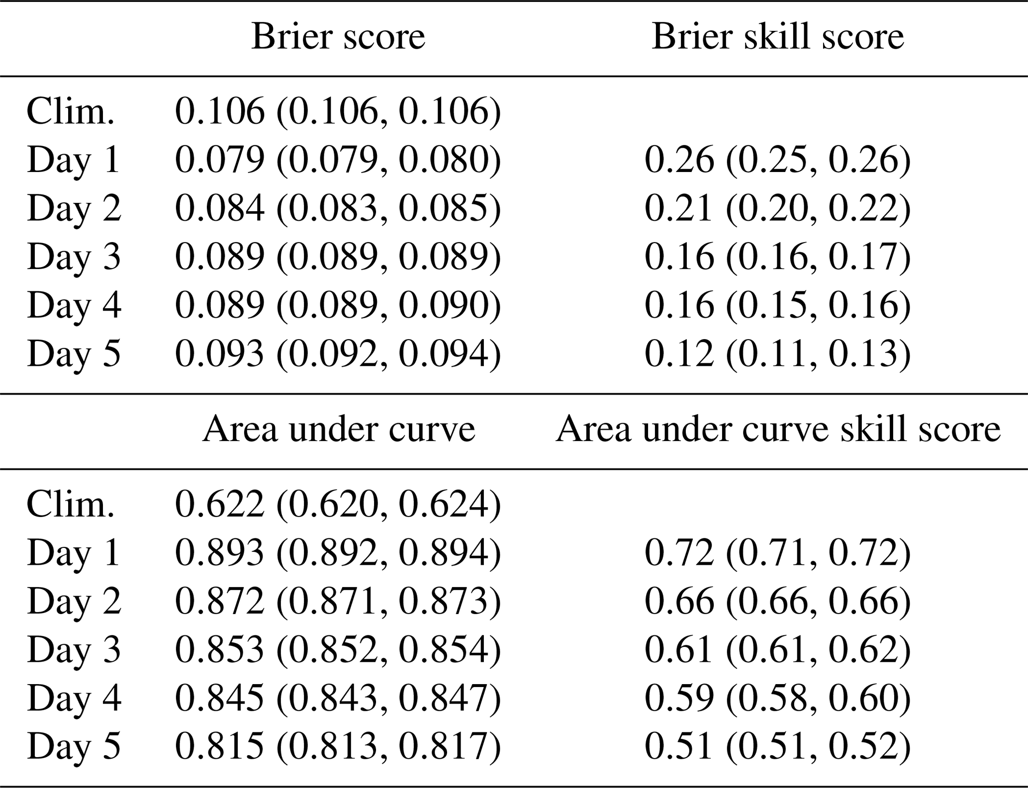
The Brier score (BS) and area under curve (AUC) derived from the receiver operating characteristics (ROC) theory are applied as verification measures. Both scores and their associated skill scores reveal that the postprocessed ECMWF predictions outperform the climatologies up to a forecast horizon of 5 days (Table 3). Inference is based on the samples from the MCMC sampling.

Table 3Out-of-sample performance of the occurrence model; 95 % credible intervals based on MCMC samples are given in parentheses.

Download Print Version | Download XLSX

Further, the Brier skill score (BSS) is investigated over space for a lead time of 5 days (Fig. 7). A 7-year climatology encompassing a spatial and seasonal effect (Eq. 2) serves as a reference forecast. The highest skill can be found in the southern half of the same domain as well as in the north-eastern region. Inference based on MCMC samples reveals significant positive skill along the main Alpine ridge. In order to account for multiple testing, due to testing each individual box, we apply the correction for controlling the false discovery rate (Benjamini and Hochberg, 1995) which is robust to spatial dependence within the field of the test (Wilks, 2016). A control level of 5 % was chosen, which leads to a threshold of 3.4 % for rejecting a local null hypothesis (see Eq. 3 in Wilks, 2016).

https://www.adv-stat-clim-meteorol-oceanogr.net/5/1/2019/ascmo-5-1-2019-f07

Figure 7Spatial distribution of Brier skill scores for a lead time of 5 days evaluating the occurrence of lightning events (no. of flashes >0). Blueish colours indicate significantly positive values.

Download

4.2.2 Intensity of lightning events

The evaluation of the predictive performance with respect to the intensity of lightning events takes the hurdle model (Eq. 1) into account. We investigate the global performance of the forecasts, firstly, by averaging scores over all grid boxes, secondly, by visualizing rootograms for a graphical portrayal of calibration, and, thirdly, by looking at the spatial distribution of skill scores.

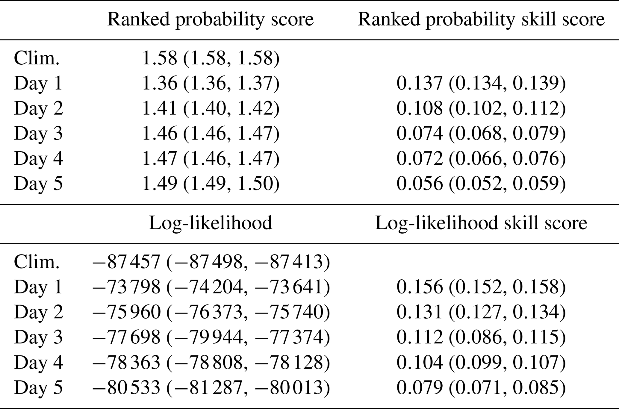
For every day a probability mass is predicted for every possible outcome $y \in {0, 1, 2, \dots}$ , which are evaluated (Table 4) with the ranked probability score (RPS, Epstein, 1969) and log-likelihood of the hurdle negative binomial distribution, i.e. the combination of the Bernoulli and zero-truncated negative binomial distribution. The predictions are compared against a reference climatology in which each parameter – π, μ, and θ – is modelled by a seasonal effect and a spatial effect. The models based on the ECMWF covariates outperform the climatology up to a forecast horizon of 5 days.

Table 4Out-of-sample performance of the intensity model; 95 % credible intervals based on MCMC samples are given in parentheses.

Download Print Version | Download XLSX

Marginal calibration of the predicted distributions is assessed by the use of rootograms (Fig. 8). Rootograms compare the observed frequencies for every possible outcome ${0, 1, 2, \dots}$ with the expected frequencies – the sum of the predicted densities over all samples – on the square root scale (Kleiber and Zeileis, 2016). In a hanging rootogram bars indicating the square root of the observed frequencies hang from a curve showing the square root of expected frequencies.

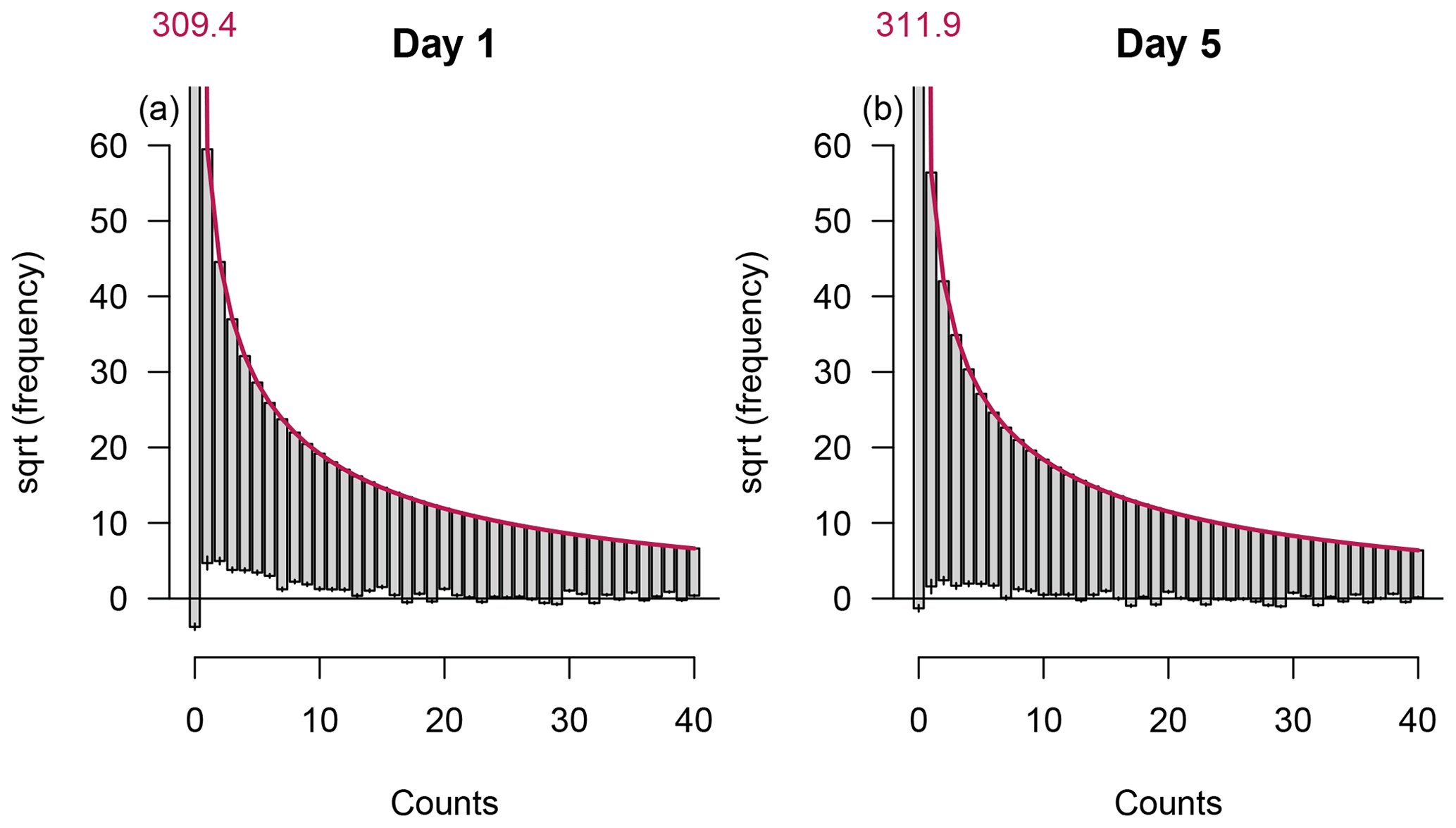
https://www.adv-stat-clim-meteorol-oceanogr.net/5/1/2019/ascmo-5-1-2019-f08

Figure 8Hanging rootograms for the intensity models with a forecast horizon of 1 and 5 days. The curve shows the expected frequencies and bars the observed frequencies on the square root scale. The small vertical lines bisecting the bottom ends of the bars show the 95 % credible intervals from MCMC sampling of the difference between expected and observed frequencies.

Download

The rootogram for day 1 reveals that the amount of zero counts is underestimated and that counts in the range from 1 to approx. 10 are overestimated. For higher counts the rootogram reveals good calibration of the model. The rootogram for the model with a forecast horizon of 5 days shows slightly better calibration for counts in the lower range. Although the bottom end of the bar for zero counts is closer to the x axis, the 95 % credible intervals from the MCMC sampling reveal that the model also underestimates the amount of zeros.

Finally, we investigate the spatial distribution of different skill scores for a lead time of 5 days (Fig. 9). From the hurdle model a probability forecast for exceeding 10 flashes per grid box, a prediction of the 90 % quantile, and the full probability distribution as prediction per se are derived. A 7-year climatology encompassing spatial and seasonal effects for the three parameters – π, μ, and θ – of the hurdle model serves as the reference forecast. The three spatial distributions of skill reveal the same pattern as the skill score of the occurrence model (Fig. 7), with the highest skill in the north-eastern corner of the domain and in the southern half which includes the main Alpine ridge. The inferential conclusion about whether skill is significantly positive in a box is based on the MCMC samples. Again, the correction for multiple testing is applied with a control level of 5 % (Wilks, 2016), which leads to thresholds of 2.6 %, 2.8 %, and 3.0 % for rejecting a local null hypothesis in the cases of the Brier, quantile, and ranked probability skill scores, respectively.

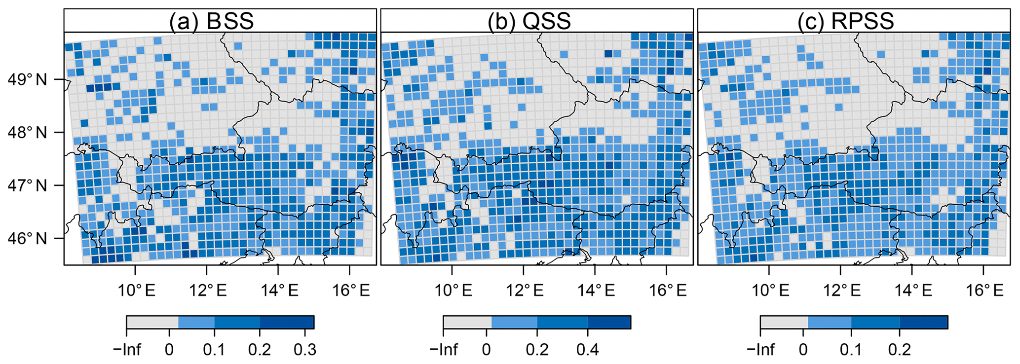
https://www.adv-stat-clim-meteorol-oceanogr.net/5/1/2019/ascmo-5-1-2019-f09

Figure 9Spatial distribution of skill scores for a lead time of 5 days. Blueish colours indicate significantly positive values. (a) Brier skill score for exceeding 10 flashes per grid box. (b) Quantile skill score for the 90 % quantile. (c) Ranked probability skill score for the full predictive distribution.

Download

5 Discussion

This section connects the present work to previous studies (Sect. 5.1) and discusses how the proposed methods can be transferred to further applications (Sect. 5.2), for which increasing the number of input variables can be crucial (Sect. 5.3). At the end of this section we summarize and conclude the study (Sect. 5.4).

5.1 Connection to other studies

We discuss the relation of the present work to two other studies: firstly, a work with meteorological background on the prediction of thunderstorm occurrence in the Eastern Alps (Simon et al., 2018). Secondly, a work from the statistical literature which focuses on gradient boosting for distributional regression and which presents a case study with a count data variable as response (Thomas et al., 2018).

Simon et al. (2018) postprocess the deterministic high-resolution (HRES) ECMWF forecast from 2010 to 2015 to predict the probability of the occurrence of thunderstorms. The methodology – stability selection with gradient boosting, and MCMC sampling – is similar to the methods applied in this study. However, the binomial model used by Simon et al. (2018) is less complex, and less computationally expensive. As counts are not considered by Simon et al. (2018), only the results of the binary hurdle are compared with their results: during 2010–2015 the native resolution of the ECMWF HRES was 16×16 km² and thus comparable to the resolution of the target variable in this study. Although the framework was different – a longer training period of 4 years and only deterministic NWP forecasts – the resulting out-of-sample scores are comparable: Brier skill score ranges from approx. 0.25 to approx. 0.12 throughout the forecast horizons of 1 to 5 days. The AUC ranges from 0.88 to 0.79. Also, the spatial patterns of the skill match with patterns presented by Simon et al. (2018). This finding suggests than the short training period of the present study covers a sufficient variety of atmospheric processes leading to lightning, which enables the statistical model to learn these processes.

Thomas et al. (2018) apply a hurdle model with a zero-truncated negative binomial in their study about abundance of wintering sea ducks. The abundance of sea ducks is quantified on a grid which leads to a response quantity with similar properties to the present lightning counts: 75 % zeros and overdispersion. They also separate the hurdle model for the selection of terms by gradient boosting with stability selection. However, in Thomas et al. (2018)'s study, terms for the dispersion parameter θ have also been selected, which could also be a consequence of less regularization within the individual boosting runs.

There is one more important difference between the present study and the work by Thomas et al. (2018), namely the way in which the final model is estimated. After the selection procedure, their final model is fitted by gradient boosting. The optimal amount of regularization – tuning the number of iterations – is found by maximizing the out-of-bootstrap log-likelihood. In the present study the final model is estimated using MCMC sampling. Thus regularization is performed for each individual term by a prior distribution. A major advantage of this Bayesian approach is that inferential conclusions for effects, scores, and predictions can be drawn from the MCMC samples.

5.2 Transfer of method

The postprocessing method presented in this study can be easily transferred to other types of lightning, e.g. total lightning, or other regions of the world. The key to this transferability is the objective selection scheme, i.e. stability selection combined with gradient boosting, which enables us to adapt the predictors to the new application. Further, implementations of the selection and MCMC sampling scheme proposed in this study are made available in the bamlss flexible regression toolbox (Bayesian additive models for location, scale, and shape (and beyond), Umlauf et al., 2018), which is an add-on package for the R software environment (R Core Team, 2018). Thus, users can easily test the proposed method on the data of their application.

The method could also be applied to a larger domain, for instance an entire continent. In the case of Europe this would lead to an increase in the area and thus in the data by at least 1 order of magnitude. The amount of data would further increase when the pool of candidate terms for the additive predictors is extended. Thus, transferring the method to a larger domain is likely to offer some challenges in data handling and efficiency of the optimization schemes.

5.3 Increasing the number of input variables

The variables that initially enter the selection procedure already cover a wide range of atmospheric processes. However, there are many variables that are promising for further improving the predictive performance of the final model. Most interesting would be to investigate the influence of parameterized lightning variables in the ECMWF output (Lopez, 2016) introduced in mid-2018 (Lopez, 2018). Further candidates are cloud properties (graupel, supercooled water, ice crystals) related to charge separation (e.g. Saunders, 2008).

In addition to variables from a NWP, observations from previous time steps could also add predictive skill. From an operational perspective, adding the lagged response increases the technical effort, as not only do data from a NWP have to be gathered, but the supply of the lightning observation for forecast production also has to be guaranteed.

The candidate pool can be further extended by variables that describe the orography in more detail, such as altitude, slope, and the orientation of the slope. This extension would especially give deeper insights into the climatological effects. At the scale of 18×18 km² we found no benefit of including orography-related covariates. However, at finer spatial scales orography-related covariates might have more influence (Simon et al., 2017).

5.4 Summary

To conclude, we summarize the methods and the key findings of this study. We propose a framework to predict the probability of occurrence and the intensity of lightning events (or thunderstorms) in the European Eastern Alps. A hurdle approach – with a Bernoulli hurdle and a zero-truncated negative binomial as count part – is chosen to account for excess zeros and overdispersion in the lightning count data. Covariates for nonlinear terms in additive predictors are derived from the ECMWF ensemble prediction system. An objective selection procedure – gradient boosting with stability selection – reduces the set of numerous terms. The final models are estimated using MCMC sampling in order to provide valid credible intervals for effects, predictions, and out-of-sample scores.

Both the occurrence and intensity models outperform a climatology up to a forecast horizon of 5 days. The predictive skill is greater over complex terrain of the Eastern Alps than over regions with fewer orographic features. This pattern can be associated with persistent forcing in regions with complex terrain such as orographic lifting, thermally induced circulations (plains–mountains, slope winds, valley winds), and lee effects (Houze, 2012).

Code availability

The statistical modelling was carried out using the R software environment (R Core Team, 2018). The bamlss add-on package (Umlauf et al., 2018) offers a flexible toolbox for distributional regression models. It allows one to perform gradient boosting via the boost() model fitting engine function and to simulate MCMC samples of the posterior distribution with the GMCMC() engine function. The countreg package (Zeileis et al., 2008) provides score functions and the hessian of the zero-truncated negative binomial distribution and the high-level rootogram() plotting function.

Data availability

ALDIS data are available on request from ALDIS (aldis@ove.at) – fees may be charged.

Appendix A: The negative binomial hurdle distribution

In this Appendix we derive the density and the log-likelihood of the hurdle model (Eq. 1). Hurdle models consist of two parts: a binary hurdle part – modelling the probability of zero vs. non-zero events – and a truncated count part – modelling the distribution of positive counts.

Hurdle models for counts were introduced by Mullahy (1986). A comprehensive overview of modelling count data is given by Cameron and Trivedi (2013). Zeileis et al. (2008) present an implementation of regression models for count data in the R software environment.

In the present study a Bernoulli distribution serves as the binary hurdle, and a zero-truncated negative binomial distribution as the truncated count part. The Bernoulli distribution has the density

\begin{matrix} (A1) & f_{BE} (z | π) = {(1 - π)}^{1 - z} \cdot π^{z}, z \in {0, 1}, \end{matrix}

which is determined by the probability π.

To derive the truncated count part, we start with the negative binomial (type 2) distribution (Cameron and Trivedi, 2013), with the density

\begin{matrix} (A2) & f_{NB} (z | μ, θ) = \frac{Γ (θ + z)}{Γ (θ) \cdot z!} \cdot \frac{μ^{z} \cdot θ^{θ}}{(μ + θ)^{θ + z}}, z \in {0, 1, 2, \dots}, \end{matrix}

where μ>0 is the expectation of the distribution, E(z)=μ, and θ>0 modifies the variance, $VAR (z) = μ + μ^{2} / θ$ , in order to account for the overdispersion in the gridded lightning observations. Small values of θ refer to strong overdispersion. When θ approaches infinity the negative binomial distribution converges towards the Poisson distribution, and the variance converges to μ which equals the expectation.

For truncating the negative binomial the probability mass at zero is redistributed towards positive values leading to the density of the zero-truncated negative binomial,

\begin{matrix} (A3) & f_{ZTNB} (y | μ, θ) = \frac{f_{NB} (y | μ, θ)}{1 - f_{NB} (0 | μ, θ)}, y \in {1, 2, \dots} . \end{matrix}

The Bernoulli distribution (Eq. A1) and the zero-truncated negative binomial (Eq. A3) are combined to obtain the hurdle model (Eq. 1). From the density of the hurdle model we can derive the log-likelihood function (which serves as objective function during optimization),

\begin{array}{l} ℓ (π, μ, θ | y) = \underset{{\tilde{ℓ}}_{BHP} (π | y)}{\underset{︸}{I_{{0}} (y) \cdot \log (1 - π) + (1 - I_{{0}} (y)) \cdot \log π}} \\ (A4) & + \underset{{\tilde{ℓ}}_{TCP} (μ, θ | y)}{\underset{︸}{(1 - I_{{0}} (y)) \cdot \log (f_{ZTNB} (y | μ, θ)),}} \end{array}

where I_{0}(y) is an indicator function which takes the value one if y equals zero, and zero otherwise. The log-likelihood is a function of the parameters π, μ, and θ. However, it can be separated additively into a function of π, ${\tilde{ℓ}}_{BHP} (π | y)$ , and a function of μ and θ, ${\tilde{ℓ}}_{TCP} (μ, θ | y)$ . Thus, during optimization the optima for the two functions can be obtained independently from each other.

In particular, ${\tilde{ℓ}}_{BHP}$ and ${\tilde{ℓ}}_{TCP}$ are equivalent to the log-likelihood of the Bernoulli distribution (Eq. A1) and the zero-truncated negative binomial (Eq. A3), respectively.

The gradients of ℓ w.r.t. the parameters π, μ, and θ are as follows:

\begin{array}{l} (A5) & \frac{\partial ℓ}{\partial π} = (1 - I_{{0}} (y)) \cdot \frac{1}{π} - I_{{0}} (y) \cdot \frac{1}{1 - π}, \\ \frac{\partial ℓ}{\partial μ} = (1 - I_{{0}} (y)) \\ (A6) & \cdot [\frac{y}{μ} - \frac{y + θ}{μ + θ} - {(\frac{θ}{μ + θ})}^{θ + 1} \cdot {(1 - {(\frac{θ}{μ + θ})}^{θ})}^{- 1}], \\ \frac{\partial ℓ}{\partial θ} = (1 - I_{{0}} (y)) \cdot [ψ_{0} (y + θ) - ψ_{0} (θ) + \log (θ) \\ + 1 - \log (μ + θ) - \frac{y + θ}{μ + θ} + {(\frac{θ}{μ + θ})}^{θ} \\ (A7) & \cdot {(1 - {(\frac{θ}{μ + θ})}^{θ})}^{- 1} \cdot (\log \frac{θ}{μ + θ} + 1 - \frac{θ}{μ + θ})], \end{array}

where ψ₀(⋅) is the digamma function.

Appendix B: Noncyclic gradient boosting

In this Appendix we illustrate the algorithm implemented for noncyclic gradient boosting tailored to the zero-truncated negative binomial distribution, i.e. the truncated count part of the hurdle model. The log-likelihood of the truncated count part ${\tilde{ℓ}}_{TCP}$ is a function of two parameters μ and θ with two associated additive predictors η_μ and η_θ, respectively. The additive predictors consist of terms $f_{*} (x_{*})$ , which are nonlinear functions f(⋅) of the covariates x (Eqs. 3 and 4).

The selection of influential terms is performed using noncyclic gradient boosting which is an iterative procedure, where in each iteration only the best fitting term is slightly updated. Generic versions of the algorithm can be found in Mayr et al. (2012) and Thomas et al. (2018). Here we illustrate the noncyclical gradient boosting algorithm tailored to the zero-truncated negative binomial:

Initially all terms in the two predictors η_μ and η_θ are set to zero, i.e. $f_{*} (x_{*}) = 0$ . Only the intercepts β_0, μ and β_0, θ are included.
Evaluate the negative gradients of the log-likelihood ${\tilde{ℓ}}_{TCP}$ w.r.t. the predictors by employing the chain rule,
$\begin{array}{l} - \frac{\partial {\tilde{ℓ}}_{TCP}}{\partial η_{μ}} = - \frac{\partial {\tilde{ℓ}}_{TCP}}{\partial μ} \cdot \frac{\partial μ}{\partial η_{μ}} \\ (B1) & with \frac{\partial μ}{\partial η_{μ}} = \frac{\partial \exp (η_{μ})}{\partial η_{μ}} = \exp (η_{μ}) = μ, \\ - \frac{\partial {\tilde{ℓ}}_{TCP}}{\partial η_{θ}} = - \frac{\partial {\tilde{ℓ}}_{TCP}}{\partial θ} \cdot \frac{\partial θ}{\partial η_{θ}} \\ (B2) & with \frac{\partial θ}{\partial η_{θ}} = \frac{\partial \exp (η_{θ})}{\partial η_{θ}} = \exp (η_{θ}) = θ, \end{array}$
for every observation, leading to a vectors of gradients. The derivations w.r.t. the parameters are given in Eqs. (A6) and (A7).
Fit low-degree-of-freedom splines for each term $f_{*} (x_{*})$ to the gradient vectors using penalized least squares estimation (Wood, 2017).
For each predictor the coefficients of the best fitting term – w.r.t. the residual sum of squares – are updated by a proportion ν, e.g. ν=0.1, leading to an auxiliary predictor,
$\begin{matrix} (B3) & {\tilde{η}}_{μ} = η_{μ} + ν \cdot f_{j} (x_{j}) and {\tilde{η}}_{θ} = η_{θ} + ν \cdot f_{k} (x_{k}), \end{matrix}$
and the intercepts within the auxiliary predictors are updated.
Every iteration is concluded by replacing the predictor whose auxiliary predictor leads to the largest improvement of the log-likelihood,
$\begin{array}{l} if {\tilde{ℓ}}_{TCP} (\exp ({\tilde{η}}_{μ}), \exp (η_{θ})) > {\tilde{ℓ}}_{TCP} (\exp (η_{μ}), \exp ({\tilde{η}}_{θ})) \\ (B4) & set η_{μ} = {\tilde{η}}_{μ} else set η_{θ} = {\tilde{η}}_{θ} . \end{array}$
Repeat steps 2–5 for a predefined number of iterations k_max or until a predefined number q of terms has been selected.

Author contributions

TS, GJM, and AZ defined the scientific scope of this study. TS performed the statistical modelling, evaluated the results, and wrote the paper. GJM supported the meteorological analysis. NU and AZ contributed to the development of the statistical methods. All the authors discussed the results and commented on the manuscript.

Competing interests

The authors declare that they have no conflict of interest.

Acknowledgements

We acknowledge the funding of this work by the Austrian Research Promotion Agency (FFG) project LightningPredict (contract no. 846620). The computational results presented have been achieved using HPC infrastructure LEO of the University of Innsbruck. Furthermore, we are grateful to the editor and two anonymous reviewers for their valuable comments. Finally, we thank Gerhard Diendorfer and Wolfgang Schulz from ALDIS for data support.

Edited by: William Kleiber
Reviewed by: two anonymous referees

References

Bates, B. C., Dowdy, A. J., and Chandler, R. E.: Lightning Prediction for Australia Using Multivariate Analyses of Large-Scale Atmospheric Variables, J. Appl. Meteor. Climatol., 57, 525–534, https://doi.org/10.1175/JAMC-D-17-0214.1, 2018. a

Benjamini, Y. and Hochberg, Y.: Controlling the False Discovery Rate: A Practical and Powerful Approach to Multiple Testing, J. Roy. Stat. Soc. B-Met., 57, 289–300, 1995. a

Brezger, A. and Lang, S.: Generalized Structured Additive Regression Based on Bayesian P-Splines, Comput. Stat. Data An., 50, 967–991, https://doi.org/10.1016/j.csda.2004.10.011, 2006. a, b

Buizza, R., Milleer, M., and Palmer, T. N.: Stochastic Representation of Model Uncertainties in the ECMWF Ensemble Prediction System, Q. J. Roy. Meteor. Soc., 125, 2887–2908, https://doi.org/10.1002/qj.49712556006, 1999. a

Cameron, A. C. and Trivedi, P. K.: Regression Analysis of Count Data, Econometric Society Monographs, Cambridge University Press, Cambridge, 2nd edn., 2013. a, b, c, d, e, f

Epstein, E. S.: A Scoring System for Probability Forecasts of Ranked Categories, J. Appl. Meteorol., 8, 985–987, https://doi.org/10.1175/1520-0450(1969)008<0985:ASSFPF>2.0.CO;2, 1969. a

Fahrmeir, L., Kneib, T., Lang, S., and Marx, B.: Regression: Models, Methods and Applications, Springer, Berlin, https://doi.org/10.1007/978-3-642-34333-9, 2013. a, b, c

Farr, T. G., Rosen, P. A., Caro, E., Crippen, R., Duren, R., Hensley, S., Kobrick, M., Paller, M., Rodriguez, E., Roth, L., Seal, D., Shaffer, S., Shimada, J., Umland, J., Werner, M., Oskin, M., Burbank, D., and Alsdorf, D.: The Shuttle Radar Topography Mission, Rev. Geophys., 45, 1–33, https://doi.org/10.1029/2005RG000183, 2007. a

Gamerman, D.: Sampling from the Posterior Distribution in Generalized Linear Mixed Models, Stat. Comput., 7, 57–68, https://doi.org/10.1023/a:1018509429360, 1997. a

Gijben, M., Dyson, L. L., and Loots, M. T.: A Statistical Scheme to Forecast the Daily Lightning Threat over Southern Africa Using the Unified Model, Atmos. Res., 194, 78–88, https://doi.org/10.1016/j.atmosres.2017.04.022, 2017. a

Gneiting, T., Balabdaoui, F., and Raftery, A. E.: Probabilistic Forecasts, Calibration and Sharpness, J. Roy. Stat. Soc. B., 69, 243–268, https://doi.org/10.1111/j.1467-9868.2007.00587.x, 2007. a

Hofner, B., Boccuto, L., and Göker, M.: Controlling False Discoveries in High-Dimensional Situations: Boosting with Stability Selection, BMC Bioinformatics, 16, 144, https://doi.org/10.1186/s12859-015-0575-3, 2015. a, b, c

Houze, R. A.: Orographic Effects on Precipitating Clouds, Rev. Geophys., 50, 1–47, https://doi.org/10.1029/2011RG000365, 2012. a

Kleiber, C. and Zeileis, A.: Visualizing Count Data Regressions Using Rootograms, Am. Stat., 70, 296–303, https://doi.org/10.1080/00031305.2016.1173590, 2016. a

Klein, N., Kneib, T., and Lang, S.: Bayesian Generalized Additive Models for Location, Scale, and Shape for Zero-Inflated and Overdispersed Count Data, J. Am. Stat. Assoc., 110, 405–419, https://doi.org/10.1080/01621459.2014.912955, 2015. a, b, c

Lang, S., Umlauf, N., Wechselberger, P., Harttgen, K., and Kneib, T.: Multilevel Structured Additive Regression, Stat. Comput., 24, 223–238, https://doi.org/10.1007/s11222-012-9366-0, 2014. a

Langhans, W., Schmidli, J., and Schär, C.: Bulk Convergence of Cloud-Resolving Simulations of Moist Convection over Complex Terrain, J. Atmos. Sci., 69, 2207–2228, https://doi.org/10.1175/JAS-D-11-0252.1, 2012. a

Lopez, P.: A Lightning Parameterization for the ECMWF Integrated Forecasting System, Mon. Weather Rev., 144, 3057–3075, https://doi.org/10.1175/MWR-D-16-0026.1, 2016. a

Lopez, P.: Promising results for lightning predictions, ECMWF Newsletter, 14–19, https://doi.org/10.21957/plz731tyg2, 2018. a

Mayr, A., Fenske, N., Hofner, B., Kneib, T., and Schmid, M.: Generalized Additive Models for Location, Scale and Shape for High Dimensional Data – A Flexible Approach based on Boosting, J. Roy. Stat. Soc. C App., 61, 403–427, https://doi.org/10.1111/j.1467-9876.2011.01033.x, 2012. a, b, c

Meinshausen, N. and Bühlmann, P.: Stability Selection, J. Roy. Stat. Soc. B, 72, 417–473, https://doi.org/10.1111/j.1467-9868.2010.00740.x, 2010. a

Mullahy, J.: Specification and Testing of some Modified Count Data Models, J. Econometrics, 33, 341–365, https://doi.org/10.1016/0304-4076(86)90002-3, 1986. a, b, c

R Core Team: R: A language and environment for statistical computing, R Foundation for Statistical Computing, Vienna, Austria, available at: https://www.R-project.org/, last access: 26 November 2018. a, b

Rigby, R. A. and Stasinopoulos, D. M.: Generalized Additive Models for Location, Scale and Shape, J. Roy. Stat. Soc. C-App., 54, 507–554, https://doi.org/10.1111/j.1467-9876.2005.00510.x, 2005. a

Saunders, C.: Charge Separation Mechanisms in Clouds, Space Sci. Rev., 137, 335–353, https://doi.org/10.1007/s11214-008-9345-0, 2008. a

Schmeits, M. J., Kok, K. J., Vogelezang, D. H. P., and van Westrhenen, R. M.: Probabilistic Forecasts of (Severe) Thunderstorms for the Purpose of Issuing a Weather Alarm in the Netherlands, Weather Forecast., 23, 1253–1267, https://doi.org/10.1175/2008WAF2007102.1, 2008. a, b

Schulz, W., Cummins, K., Diendorfer, G., and Dorninger, M.: Cloud-to-Ground Lightning in Austria: A 10-Year Study Using Data from a Lightning Location System, J. Geophys. Res., 110, D09101, https://doi.org/10.1029/2004JD005332, 2005. a, b

Simon, T., Umlauf, N., Zeileis, A., Mayr, G. J., Schulz, W., and Diendorfer, G.: Spatio-temporal modelling of lightning climatologies for complex terrain, Nat. Hazards Earth Syst. Sci., 17, 305–314, https://doi.org/10.5194/nhess-17-305-2017, 2017. a, b

Simon, T., Fabsic, P., Mayr, G. J., Umlauf, N., and Zeileis, A.: Probabilistic Forecasting of Thunderstorms in the Eastern Alps, Mon. Weather Rev., 146, 2999–3009, https://doi.org/10.1175/MWR-D-17-0366.1, 2018. a, b, c, d, e, f, g, h, i, j

Thomas, J., Mayr, A., Bischl, B., Schmid, M., Smith, A., and Hofner, B.: Gradient Boosting for Distributional Regression: Faster Tuning and Improved Variable Selection via Noncyclical Updates, Stat. Comput., 28, 673–687, https://doi.org/10.1007/s11222-017-9754-6, 2018. a, b, c, d, e, f

Umlauf, N., Klein, N., and Zeileis, A.: BAMLSS: Bayesian Additive Models for Location, Scale and Shape (and Beyond), J. Comput. Graph. Stat., 27, 612–627, https://doi.org/10.1080/10618600.2017.1407325, 2018. a, b, c, d, e, f

Wilks, D. S.: “The Stippling Shows Statistically Significant Grid Points”: How Research Results are Routinely Overstated and Overinterpreted, and What to Do about It, B. Am. Meteorol. Soc., 97, 2263–2273, https://doi.org/10.1175/BAMS-D-15-00267.1, 2016. a, b, c

Wood, S. N.: Generalized Additive Models: An Introduction with R, Texts in Statistical Science, Chapman & Hall/CRC, Boca Raton, 2nd edn., 2017. a, b, c, d, e, f

Zeileis, A., Kleiber, C., and Jackman, S.: Regression Models for Count Data in R, J. Stat. Softw., 27, 1–25, https://doi.org/10.18637/jss.v027.i08, 2008. a, b

Note that this technical term differs from overdispersion used for a predictive distribution that is too wide in the context of verifying probabilistic weather forecasts (Gneiting et al., 2007).

Articles

Short summary

Lightning in Alpine regions is associated with events such as thunderstorms, extreme precipitation, high wind gusts, flash floods, and debris flows. We present a statistical approach to predict lightning counts based on numerical weather predictions. Lightning counts are considered on a grid with 18 km mesh size. Skilful prediction is obtained for a forecast horizon of 5 days over complex terrain.