Downscaling probability of  long heatwaves based on seasonal mean daily maximum temperatures

Benestad, Rasmus E.; van Oort, Bob; Justino, Flavio; Stordal, Frode; Parding, Kajsa M.; Mezghani, Abdelkader; Erlandsen, Helene B.; Sillmann, Jana; Pereira-Flores, Milton E.

doi:https://doi.org/10.5194/ascmo-4-37-2018

Articles | Volume 4, issue 1/2

https://doi.org/10.5194/ascmo-4-37-2018

Articles | Volume 4, issue 1/2

05 Dec 2018

| 05 Dec 2018

Downscaling probability of long heatwaves based on seasonal mean daily maximum temperatures

Rasmus E. Benestad, Bob van Oort, Flavio Justino, Frode Stordal, Kajsa M. Parding, Abdelkader Mezghani, Helene B. Erlandsen, Jana Sillmann, and Milton E. Pereira-Flores

Abstract

A methodology for estimating and downscaling the probability associated with the duration of heatwaves is presented and applied as a case study for Indian wheat crops. These probability estimates make use of empirical-statistical downscaling and statistical modelling of probability of occurrence and streak length statistics, and we present projections based on large multi-model ensembles of global climate models from the Coupled Model Intercomparison Project Phase 5 and three different emissions scenarios: Representative Concentration Pathways (RCPs) 2.6, 4.5, and 8.5. Our objective was to estimate the probabilities for heatwaves with more than 5 consecutive days with daily maximum temperature above 35 ^∘C, which represent a condition that limits wheat yields. Such heatwaves are already quite frequent under current climate conditions, and downscaled estimates of the probability of occurrence in 2010 is in the range of 20 %–84 % depending on the location. For the year 2100, the high-emission scenario RCP8.5 suggests more frequent occurrences, with a probability in the range of 36 %–88 %. Our results also point to increased probabilities for a hot day to turn into a heatwave lasting more than 5 days, from roughly 8 %–20 % at present to 9 %–23 % in 2100 assuming future emissions according to the RCP8.5 scenario; however, these estimates were to a greater extent subject to systematic biases. We also demonstrate a downscaling methodology based on principal component analysis that can produce reasonable results even when the data are sparse with variable quality.

Download & links

Article (PDF, 3303 KB)

Supplement (9142 KB)

Download & links

Article (3303 KB)
Supplement (9142 KB)
BibTeX
EndNote

How to cite

How to cite.

Dates

Received: 15 Jun 2018 – Revised: 12 Oct 2018 – Accepted: 27 Nov 2018 – Published: 05 Dec 2018

1 Introduction

1.1 Weather statistics and society

People have learnt to cope with climate variations and severe weather over historical times and have adapted to various weather-related risks. In this respect, climate can be regarded as the statistical description of various weather variables (Benestad et al., 2017 a), giving a picture of “typical” types of weather and what to expect. This statistical description includes the mean, variance, autocorrelation, periodicity, and duration of various climatological events. Weather-related risks are a product of probability and consequence, where the probability is provided by the statistical distribution or a probability density function (pdf). The statistical character of weather is influenced by physical processes, and variations and changes to the climate can be linked to a number of physical conditions. Some of the most severe types of past weather-related events affecting society have included harvest failures due to cold summers or prolonged droughts (Iizumi and Ramankutty, 2015; Kumar et al., 2006; Neumann and Kington, 1992). For the case of droughts, one important statistic is their duration, even though high temperature and winds are contributing factors in terms of water stress. Likewise, the duration of events matters for livelihoods when there are periods with temperature below, above, or within a range of thresholds. For example, local statistical temperature characteristics control the prospects for various aspects of society, such as wheat crops in India, typical skiing conditions in Norway, or heatwave risks in continental Europe.

It is often tricky to estimate durations defined by a variable crossing threshold values, especially if it is based on models which are subject to biases and systematic errors (Chen et al., 2012; Maraun et al., 2010). It is also impossible to provide a detailed forecast into the far future, but statistical properties, such as the parameters describing the shape of a pdf, are more predictable than single events. Some statistical parameters tend to respond more systematically to changes in physical conditions, while others are insensitive. One trivial illustration is that the mean temperature exhibits a clear dependency on conditions such as the seasonal cycle, latitude, and altitude, whereas its autocorrelation is not very sensitive to such factors (Benestad et al., 2016). The mean seasonal temperature lends itself to climate change projections; provided that the daily temperature anomalies follow a normal distribution, it is also expected to affect the statistics of hot spell duration (here we use “hot spell” and “heatwave” as synonyms). One strategy for estimating durations of episodes, therefore, is to make use of statistical models to estimate statistical characteristics.

Sivakumar (1992) used an empirical distribution function to analyse the dry spell lengths over western Africa and found a relationship that may be used for predictions of the average frequency of dry and wet spells based on the mean annual rainfall. Lana et al. (2008) analysed the duration of dry spells over the Iberian Peninsula, assuming the spell duration statistics could be approximated by a Weibull distribution, and found decreasing trends in the length of wet intervals. A similar strategy was used in a study to estimate the number of rain-on-snow events over Svalbard (Hansen et al., 2014), although the statistic was a count of occurrences rather than the duration of intervals. The statistics of counts and duration (e.g. a streak of dry days) follow different types of distributions, where the former is expected to behave more like a Poisson process (Poisson distribution) and the latter is expected to follow the geometric distribution (Wilks, 1995). Furrer et al. (2010) pioneered the use of statistical theory for heatwaves and proposed a statistical framework to model the frequency, duration, and intensity of heatwaves. Making use of the expected characteristics of stochastic processes, they used a Poisson distribution to describe the frequency (number) of events, the geometric distribution to estimate the number of consecutive days (duration), and a generalised Pareto distribution to quantify their intensity. They applied the statistical framework to analyse trends in heatwave statistics in three temperature records from Phoenix (Arizona, USA), Fort Collins (Colorado, USA), and Paris (France). Keellings and Waylen (2014) analysed the variability of heatwaves over Florida, both in space and time, and reported both that there is considerable spatial variability in heatwave characteristics and that heatwaves have become increasingly frequent and intense throughout Florida. They made use of extreme-value analysis to quantify the heatwave intensity, the Poisson distribution to describe the number of heatwaves, and the geometric distribution to estimate their duration. Wang et al. (2015) used the statistical framework proposed by Furrer et al. (2010) and bias-corrected temperatures from a 30-member ensemble of global climate models for the projection of heatwave statistics in China. Global climate models, however, are not designed to represent local climate characteristics accurately, and it is therefore common to downscale the model output in order to get a description that is representative of the regional and local features (Benestad, 2016; Schubert, 1998; Storch et al., 1993; Wilby and Wigley, 1997). However, there have not been many studies on changes in the probability of future heatwaves based on the downscaling of large multi-model ensembles in general, and particularly not in India, where good-quality open-access data are scarce. Furthermore, we are not aware of any previous attempts to downscale the duration statistics by means of empirical-statistical downscaling (ESD). While the statistics for frequency or duration is more straightforward, as their respective distributions rely on single-parameter distributions related to the mean number or duration, extreme-value distributions are trickier since they involve several parameters with a less clear connection to large-scale conditions.

Here we apply the methodology for downscaling duration statistics to examine critical temperatures for growing wheat in India, which vary between the different phenological stages. The mean duration of hot spells with temperature above a critical threshold has an important effect on agriculture, especially if the statistics of duration follow a geometric distribution for which the mean is directly connected to the parameter that sets the shape of the pdf. The probability of lasting hot spells with a duration exceeding a given threshold in the current climate can be inferred from statistical properties found in the observations. An important question is how global warming will lead to more long-lasting hot spells with a detrimental effect on the wheat crops. A novel aspect of the strategy presented in this paper is the downscaling of probabilities directly, rather than downscaling a physical variable and then using it to estimate the parameters for the pdf.

1.2 Consequences of temperature on agriculture

Wheat is one of the major crops in India, and the largest wheat growing regions are in the Indo-Gangetic Plain (IGP) – particularly in the north-western states Uttar Pradesh, Punjab, Haryana, and Rajasthan (Lobell et al., 2012 b) – and in the central state Madhya Pradesh (Directorate of Economics and Statistics, 2017) in addition to Bihar in the north-east. In these states, wheat is grown over the winter season, sown between mid-November (north-west) and mid-December (central), and harvested in late March to mid-April. While this period is typical for the variety known as winter wheat, the main variety that is grown during this period is spring wheat. Wheat goes through three distinct growing and maturation phases, from the vegetative phase from germination and seedling development (1); through a reproductive phase with branching, elongation, and heading (2); to a flowering, grain setting and filling, and maturation phase (3).

Wheat is differentially temperature sensitive across its various development stages and through different mechanisms, and effects on growth or yield are gradual and variety specific. Porter and Gawith (1999) summarised from many studies non-lethal temperatures for wheat in the range of 18 to 47 ^∘C, but this covers a broad range of world cultivars across several growing stages. Wheat and any other plants grow and develop within thermal limits called cardinal temperatures. These limits characterise a Gaussian curve with the extreme points and a narrow range of temperatures where the morphophysiological (relating to, or concerned with, biological interrelationships between form and function) events are maximal, and hence termed the optimum temperature range “top”. After this range, the minimum basal temperatures “T_min” and maximum “T_max” are found, after which growth and morphophysiological activity are paralysed by deficiency and excess of energy, respectively.

It is generally accepted that optimal temperatures for wheat are in the range 17–23 ^∘C over the entire growing season, with a T_min of 0 ^∘C and T_max of 37 ^∘C, beyond which growth stops Porter and Gawith (1999).

In India, there are many varieties of wheat grown across the states, differing in their sensitivity to temperatures and other parameters, and there are also breeding programmes for heat tolerance (Mishra et al., 2014; Saxena et al., 2016). Across its various growth stages, the national recommendations for wheat growth (Directorate of wheat development, 2015) state a daily average between 20 and 25 ^∘C as optimal temperature. Critical minimum temperatures are around 3.5–5.5 ^∘C, and the maximum around 35 ^∘C. Temperatures above the optimum (25 ^∘C) lead to decreased grain yields, and temperatures above 30 ^∘C at maturity (around mid-March) lead to forced maturity and yield loss. Warming is already affecting wheat yields across the world, and for each degree increase in global mean temperature, there is a reduction in global wheat grain production of about 6 % (Asseng et al., 2015).

For some wheat varieties, the first and second growing phases benefit from cold exposure known as vernalisation, which improves yield by shortening the duration to flowering, and thus leave more time to grain formation and filling before high temperatures set in (Sharma et al., 2012). Vernalisation is not critical to yield per se, and the duration and temperature requirements (chill-degree days) differ for different winter wheat types (McMaster et al., 2008).

For all Indian wheat varieties, the main challenge is the high temperatures in the final growing phase, late in the season from February to April (Asseng et al., 2011; Lobell et al., 2012 a). The most temperature-susceptible reproductive stages are the period priors to flowering and during flowering and fertilisation (Luo, 2011 b). Extremely high temperatures drastically affect wheat during the reproductive phase, particularly during pollination, but there is no evidence of the temperature effect on the leaf area and the production of vegetative biomass. The harmful effect on the reproduction and grain filling under high temperatures conditions intensifies with dry events during the spring or summer (Barlow et al., 2015; Hatfield and Prueger, 2015), which is the period where the phases of reproduction and grain filling occur preferentially (Luo, 2011 a).

There does not seem to be a consensus between studies on the exact critical temperature limits, and the effects of increasing temperature on yield appear to be gradual. Signs of thermal shock proteins have been found in several wheat varieties in the vegetative and reproductive phase, suggesting that they were able to extend their tolerance limits to high temperatures through genetic breeding (Krishnan et al., 1989; Xue et al., 2013). Three days of 30 ^∘C showed a reduction of grain set by almost 70 % (Saini and Aspinall, 1982), and temperature regimes of 36 and 31 ^∘C (day and night, respectively) for 2 days resulted in 55 %–85 % grain sterility (Tashiro and Wardlaw, 1990). Tiwari et al. (2017) suggested 30 ^∘C as an upper limit (daily maximum temperature T_max) around the flowering period as short periods (4 days) above this limit impact yield. Lobell et al. (2012 b) similarly found that temperatures above 30 ^∘C slow grain filling, damaging the plant. Other studies (Rao et al., 2015) have suggested higher critical temperatures: an exposure to daily T_max above 36 ^∘C and T_min 31 ^∘C during the period immediately before flowering (January) may result in sterility and reduced yield. Simulated yield studies show possible reductions of about 10 %–15 % by the end of the century if 40 ^∘C is exceeded for only 1 day (Koehler et al., 2013).

Several studies (Duncan et al., 2015; Rao et al., 2015) have found that wheat is becoming more sensitive to increasing minimum temperatures and that a continuous exposure to a daily minimum temperature (T_min) exceeding 12 ^∘C for 6 days and T_max exceeding 34^∘C for 7 days past flowering (February) constrains yields (Rao et al., 2015).

In summary, the period February–April is most critical, with all temperatures above optimal decreasing wheat yield. Studies on the more sensitive varieties suggest a daily maximum in February of 30 ^∘C as a limit above which yield is reduced. However, to simplify the analysis, the threshold for maximum temperature before limiting wheat crop yields was set to 35 ^∘C for 5 consecutive days based on published research (Saini and Aspinall, 1982; Tashiro and Wardlaw, 1990). Based on this information, our objective was to estimate the likelihood for long-lasting future heatwaves with detrimental consequences for Indian wheat production. We explored a new methodology within downscaling, making use of large multi-model ensembles to get an ad hoc representation of uncertainties associated with interannual-to-decadal variability and model differences.

2 Method & data

2.1 Method

The probability of long-lasting heatwaves (with $T_{max} \geq 35$ ^∘C lasting 5 days or more) was estimated through a chain of dependencies, starting from (1) different emission scenarios and continuing to (2) different climate sensitivities to the global response simulated by global climate models, (3) the local mean temperature, (4) the mean duration of heatwaves, and (5) the probability of duration longer than some critical length. Here, we present a strategy for the last three. We also took into account the first two by using simulations with different global climate models and emission scenarios.

2.1.1 Hypotheses

Our main working hypothesis ℋ₁ was that the seasonal mean hot spell duration $\overline{L_{H}}$ exhibits a predictable and universal dependency on the seasonal mean daily maximum temperature $\overline{T_{max}}$ . In other words, the link between the mean values of the two distributions for daily maximum temperature and the hot spell duration was analysed, rather than the link between the mean and extreme statistics. We also looked at a subsidiary hypothesis ℋ₂: that the length of the hot spells follows a geometric distribution in terms of number of days with $Pr (L_{H} = k) = (1 - p)^{(k - 1)} p$ (k=1, 2, 3,…) for which the mean duration is the inverse of the probability of a hot day $\overline{L_{H}} = 1 / p$ . If these two hypotheses can be verified, then it may be possible to make use of projections for seasonal mean temperature to estimate changes in the hot spell duration statistics. Such calculations may provide useful information for decision-making concerning agriculture, wheat crops, and which cultivars may be needed in the future.

One obstacle to such analyses was the poor data availability and quality over India, which restricted our ability to extract representative numbers for the hot events and connect these to climate model projections. We made use of additional information concerning mean temperatures and spell length statistics to support the analysis, which included using “high-quality” European data from the European Climate Assessment and Dataset (ECA&D; Klein Tank et al., 2002) and synthetic data prescribed with a normal distribution. We assumed that the relationship between the mean spell duration $\overline{L_{H}}$ and the seasonal mean daily maximum temperature $\overline{T_{max}}$ is a universal trait that is valid in both India and Europe (hypothesis ℋ₁) if the statistics for daily seasonal temperature anomalies can be approximated by a normal distribution with an approximately invariant variance σ². This assumption was tested over Europe by comparing the geographical distribution in winter mean temperature with mean cold spell (freezing temperatures) lengths as well as the corresponding summer mean temperature and mean warm spell length (days with daily maximum temperatures above 20 ^∘C; see Supplement). A general linear model (GLM) was used to calibrate an approximate relation between the seasonal mean temperature and the seasonal mean spell duration (Dobson, 1990; McCullagh and Nelder, 1989); the results of this analysis are presented in Fig. 1. The test was also applied to the temporal domain for long time series by comparing interannual variations in winter and summer mean temperature and the corresponding mean spell lengths. To support the analysis based on the observed temperature with synthetic data, we used a Monte Carlo simulation which by design was set to be Gaussian AR(1) noise with a autocorrelation of 0.7 to match the observations (similar to 0.8 as reported by Benestad et al. (2016) for daily mean temperatures; see Fig. 1).

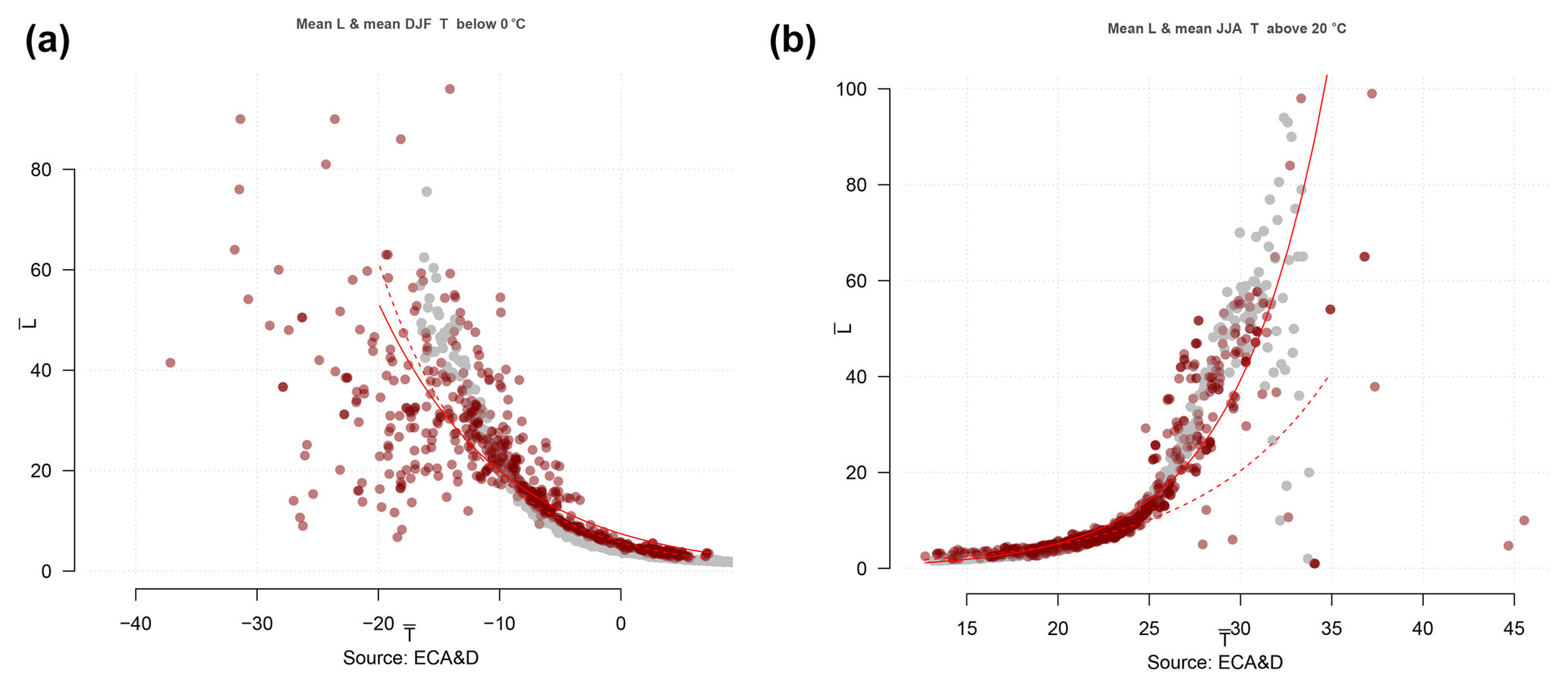
https://www.adv-stat-clim-meteorol-oceanogr.net/4/37/2018/ascmo-4-37-2018-f01

Figure 1Comparison between winter (a) and summer (b) mean daily maximum temperature (x axis) and the mean duration of cold (a) or warm (b) spells in Europe based on ECA&D. Grey dots show comparable results to a set of Monte Carlo simulations carried out with Gaussian red noise, and red lines indicate best fits based on GLM with a negative binomial (dashed lines) and a Poisson-type GLM (solid lines). The GLMs fit were statistical significant at the 1 % level for both cases (see Supplement).

Download

Given a dependency between the mean temperature and the mean spell duration (ℋ₁), the next step was to test whether the spell lengths followed a geometric distribution (ℋ₂). For this purpose, a quantile–quantile plot was used to compare the statistics of spell duration to the geometric distribution.

We present two types of probability estimates here: (1) $Pr (n_{H} \geq 1 | L_{H} > 5, T_{max} > 35$ ^∘C), the probability of at least one heatwave event lasting more than 5 days during a season, and (2) Pr(L_H>5d), the probability of a heatwave lasting longer than 5 days. The latter probability estimates are based on the two hypotheses ℋ₁ and ℋ₂. This is the same mathematical framework for analysing the frequency of events and their duration as in Furrer et al. (2010), Keellings and Waylen (2014), and Wang et al. (2015), although we did not need the statistics of the intensity for heatwaves and, hence, did not need the general extreme-value theory to model the intensity.

The probability of at least one event in a season (probability type 1) was estimated based on a statistical model assuming the Poisson distribution conditioned by the seasonal mean maximum temperature. Rather than using a GLM calibrated on individual events for each season, we used an ordinary linear regression (OLR) to predict the mean number of events $\overline{n_{h 5}}$ based on the seasonal mean maximum temperature for the entire record at each location. The reason for this choice was that the mean estimate was approximately normally distributed and that this aggregation reduced the effect of outlying seasons. The OLR also gave results that were in closer agreements with the observed frequencies.

To estimate the probability of a 5-day or longer heatwave (probability type 2), the projections of seasonal mean maximum temperature were used together with a GLM calibrated on daily maximum temperature data to infer changes in the mean hot spell duration length ( $T_{max} > 35$ ^∘C). The historical distribution of hot spell duration for the individual events approximately followed the geometric distribution, which has one parameter describing the pdf: the mean $\overline{L_{H}} = 1 / p$ . The geometric distribution was then used to estimate probabilities Pr(L_H>5d), given estimates for the mean duration $\overline{L_{H}}$ . We estimated the seasonal mean duration through a GLM and the seasonal mean temperature.

2.1.2 Temperature projections

We used ESD to make future projections for the February–April mean daily maximum temperature for a set of locations in India (see the Supplement for map) with multi-model ensembles as in Benestad et al. (2016): 108 runs of the intermediate-emission scenario Representative Concentration Pathway (RCP)4.5, 81 runs of the high-emission scenario RCP8.5, and 65 runs of the low-emission scenario RCP2.6. Using large multi-model ensembles gave more robust results and alleviated limitations caused by small sample sizes and “the law of small numbers” (Kahneman, 2012) due to larger sampling fluctuations with smaller samples (Benestad et al., 2017 b). A principal component analysis (PCA) was used to represent the local temperature (predictands) in order to enhance the signal-to-noise ratio (Benestad et al., 2015 a), and the ESD model involved a stepwise multiple linear regression where the predictand was represented by PCAs describing the February–April mean maximum temperature $\overline{T_{max}}$ . The predictors were common empirical orthogonal functions (Benestad, 2001) estimated from combined temperature anomalies from the ERA-40 reanalysis (Simmons and Gibson, 2000) and respective general circulation models (GCMs). One ESD model was calibrated for each of the five leading PCAs of $\overline{T_{max}}$ , which together accounted for 100 % of the variance. The skill of the downscaling was validated in terms of the correlation of a 5-fold cross-validation (Gutiérrez et al., 2018) and as an ensemble as a whole (Benestad et al., 2016). To obtain a starting point for estimating the probabilities, we used the median q₅₀ of the multi-model ensemble as the threshold for Pr(X>x), equivalent to a 1-in-2-year event ( $Pr (X > q_{50}) = 0.5$ ).

We used the mathematical framework described in the previous section to analyse the probability of events and their duration. To obtain projections of the probability of one or more heatwaves ( $T_{max} > 35$ ^∘C exceeding 5 days) in a season (probability type 1), we used the established dependency (OLR) between the seasonal mean maximum temperature and the mean number of events over the entire data record, and applied it to the downscaled February–April mean daily maximum temperatures. Similarly, the projections of seasonal mean maximum temperature were used together with a GLM calibrated on seasonal mean daily maximum temperature data and mean heatwave length on a season-to-season basis (i.e. aggregated from small samples) to infer changes in the mean hot spell duration length and the probability of a hot event lasting more than 5 days (probability type 2).

To produce maps of probabilities, the results were gridded using the same kriging method as in Benestad et al. (2016). The method was based on the LatticeKrig package (Nychka, 2014), taking a “fixed-rank kriging” approach with a large number of basis functions to provide spatial estimates that were comparable to standard families of covariance functions. We used elevation as a co-variable in the gridding. The gridding was only included in the final stage of the analysis, as the regression analysis and the downscaling were first applied to station records or PCAs to compute the various statistics.

In summary, this downscaling study brings in several novel aspects, including utilising large multi-model ensembles of GCM simulations, downscaling essential statistical characteristics of heatwave durations, and producing outlooks for the probability of future heatwaves lasting more than 5 days. These results were based on PCA of the local temperatures, which enhances the signal and can make the results more robust for a situation where the data are both scarce and considered to be of questionable quality.

2.2 Data

The daily maximum temperature T_max from India was obtained from the Global Historical Climate Network (GHCN) data set (Menne et al., 2012 a, b) through the R package esd (Benestad et al., 2015 b). The analysis was applied to aggregated statistics, the mean daily maximum temperature over a season $\overline{T_{max}}$ , rather than daily values. We only analysed the season important for wheat, in this case February–April, but the method described here could also be suitable for other choices. The station data were weeded to exclude locations with short data records (only keeping more than 10 290 valid daily temperatures in the interval 1970–2015), resulting in 35 station records (see map in the Supplement). To support the analysis for India and test the veracity of the identified links between the mean and the spell duration statistics, we also included data from the ECA&D data set (Klein Tank et al., 2002). The ECA&D data included 656 stations in Europe with more than 1000 days above 20 ^∘C (used to define a warm day in summer) or below 0 ^∘C (used to identify a cold day in winter) and represented a significantly greater volume of data than the temperature records for India obtained from GHCN.

More details about the data, processing, and analysis are provided in the Appendix and the Supplement, which provide results from an R Markdown script, available from figshare (Benestad, 2018) together with necessary data. The R Markdown script provides complete instructions for repeating the analysis presented here, and much of the data processing and handling were carried out with the R package esd (Benestad et al., 2015 b) (version 1.7072).

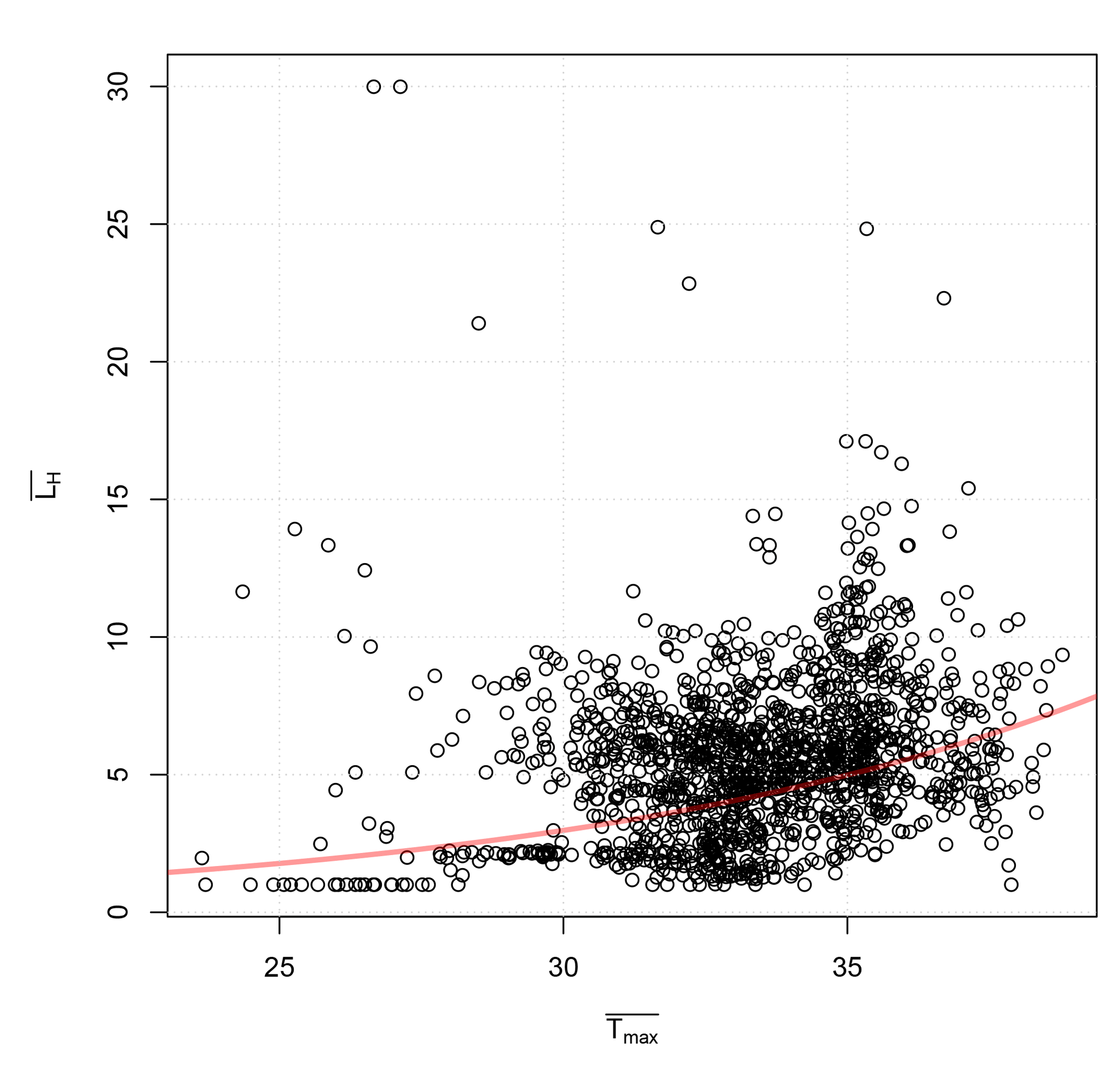
https://www.adv-stat-clim-meteorol-oceanogr.net/4/37/2018/ascmo-4-37-2018-f02

Figure 2A comparison between interannual and geographical variations in the mean duration $\overline{L_{H}}$ of hot ( $T_{max} > 35$ ^∘C) spell length from Indian temperature records and the February–April mean daily maximum temperature $\overline{T_{max}}$ . The red line marks results from a GLM model assuming a negative binomial process. Each data point represents the paired ( $\overline{L_{H}}$ , $\overline{T_{max}}$ ) for the 35 different locations and for each year during 1970–2015 (i.e. 1505 data points). The fit accounted for 10 % of the variance and was statistically significant on the 1 % level (see Supplement).

Download

3 Results

An evaluation of the downscaled results for the February–April mean maximum temperature $\overline{T_{max}}$ suggested high skill for the leading PCA in terms of the cross-validation, with correlations in the range 0.79–0.87 (Supplement). When the downscaled results for the PCAs were used to recover the format of the original temperature records, an evaluation of the RCP4.5 ensemble indicated good skill for $\overline{T_{max}}$ over the wheat growing IGP region, but low skills in the south (Supplement). The skill of downscaling was low for the stations in southern India, as both the trends in the downscaled results and the range of interannual variability were lower than seen in the observations over the common overlapping period (1970–2015). The differences in skill can be explained from the leading PCA, which had strongest weights for the locations with high skill and weakest weights where the skill was low.

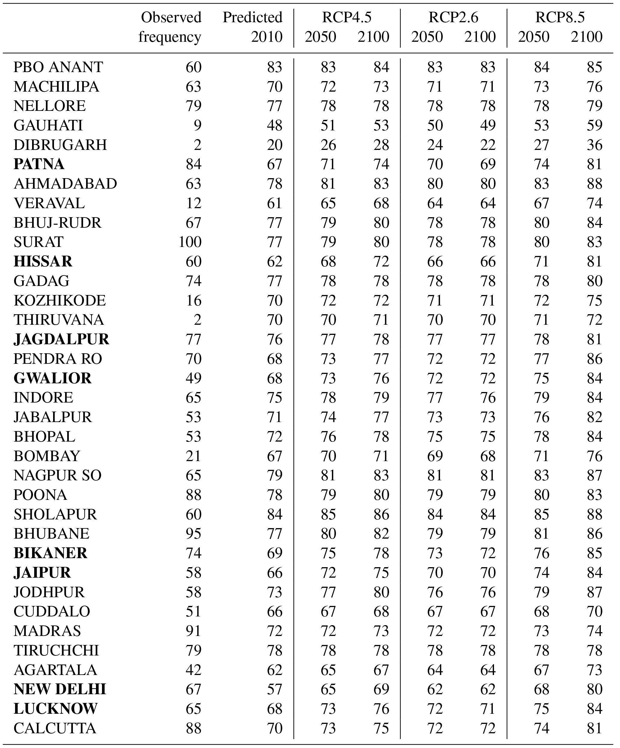
Table 1Estimated probability (expressed in %) for an episode with temperatures exceeding 35 ^∘C over more than 5 consecutive days in February–April. The observed frequency was based on the individual observational record and length of time series, and it is not exactly equivalent to the estimated probability for 2010. The location names in bold font mark stations within the IGP region.

Download Print Version | Download XLSX

An evaluation of the OLR used to estimate the mean number of heatwaves for the different sites suggested a statistically significant dependency on the seasonal mean daily maximum temperature at the 1 % level, with an R² of 0.2 (Supplement). There was a great deal of scatter about the fitted line, which suggests that there may be other important factors or that the data have variable quality.

In order to trust the results and analysis presented for the duration of the heatwaves, we also needed to test the underlying assumptions about the statistical nature of the data (ℋ₁ and ℋ₂). The first assumption was that the temperature is approximately normally distributed and that there is a systematic dependency between the mean duration of hot episodes and the mean temperature (ℋ₁). We tested this dependency by looking at the best available data (ECA&D data from European stations), assuming that the way $\overline{L_{H}}$ depends on $\overline{T_{max}}$ is a universal property for daily temperatures on Earth that is close to the dependency found for data with a normal distribution. Figure 1 shows one set of test results for the relationship between the mean seasonal temperature and mean duration of cold spells in winter and warm spells (with $T_{max} > 20$ ^∘C) in summer over Europe. The observational data (red symbols) are shown together with results from an analysis repeated with synthetic normally distributed data (grey). The results of this test confirmed the systematic dependency of the mean spell duration on the seasonal mean temperature. The results from a similar test on data from India were consistent with these results, albeit with a smaller statistical sample and a substantial scatter (Fig. 2). The fitted curve could account for 10 % of the variance according to an analysis of variance, and the results were statistical significant at the 1 % level.

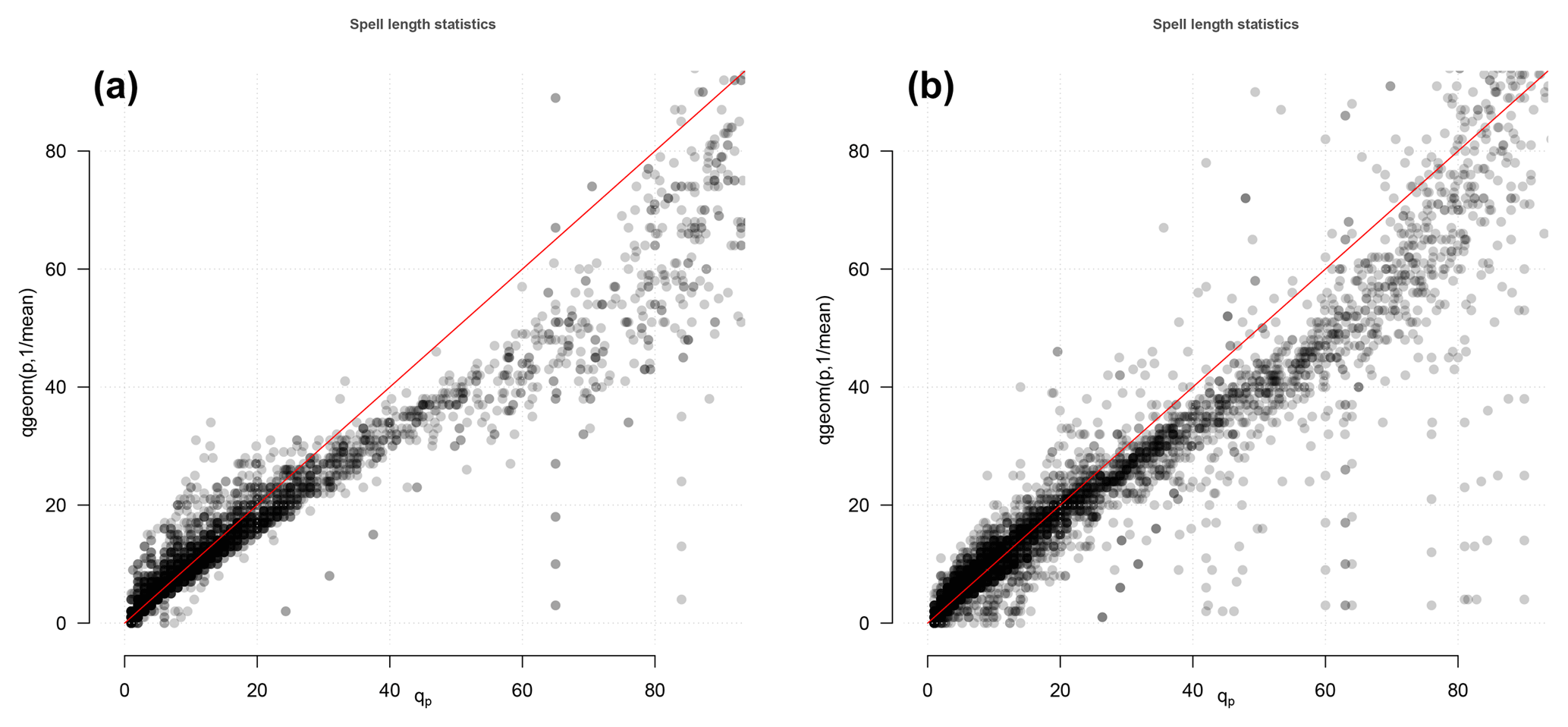
https://www.adv-stat-clim-meteorol-oceanogr.net/4/37/2018/ascmo-4-37-2018-f03

Figure 3Quantile–quantile plot between the cold (a) and warm (b) spell length and the fitted geometric distribution for the selected ECA&D stations.

Download

The second assumption was that the spell duration statistics had a geometric distribution (ℋ₂). Figure 3 shows a comparison between the spell duration statistics based on the European ECA&D data and the geometric distribution as a quantile–quantile plot. The results suggested that the assumption of a geometric distribution was reasonable for short-to-moderate duration but not for durations longer than a single season (90 days). For the case of summer, the duration statistics exhibited a high bias for durations greater than 30 days. The tests of the underlying assumptions suggested that they were reasonable for both warm and cold seasons at least in Europe. A comparison between histograms of heatwave durations in India and fitted geometric distributions based on $\overline{L_{H}}$ suggested a reasonable match (Supplement). The evaluation of hypotheses ℋ₁ and ℋ₂ provided support for making projections of the probabilities based on the ESD of $\overline{T_{max}}$ from large multi-model ensembles. A summary of the results of the probability projections are found in Tables 1 and 2. The estimated probability of at least one heatwave in a February–April season predicted for the present day (2010) was in a reasonable agreement with the observed frequency of events for most stations, but there were some exceptions where the modelled estimates were substantially higher than the observed frequency (first two columns in Table 1). However, none of these exceptions affected the stations in the IGP region (bold font in Table 1.) The sites with a mismatch between the observed frequency and estimated probability will be discussed further later on.

Table 2Estimated probability (expressed in %) for duration greater than 5 consecutive days with temperatures exceeding 35 ^∘C during February–April. The observed frequency was based on the number of February–April heatwaves lasting more than 5 days divided by the total number of heatwaves in February–April. The location names in bold font mark stations within the IGP region.

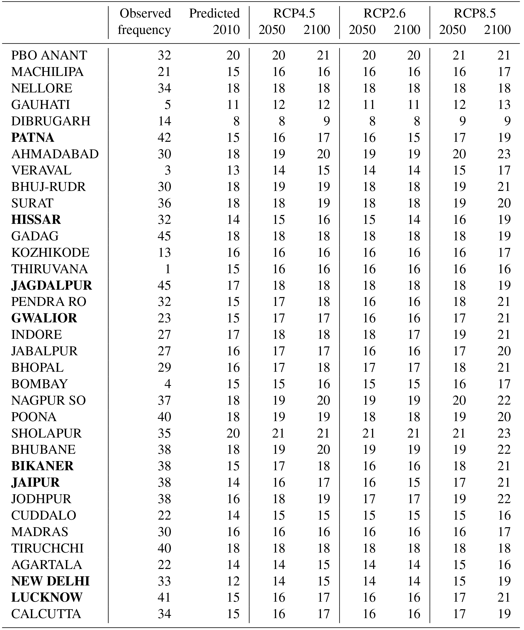
Download Print Version | Download XLSX

The projected probability of a hot event ( $T_{max} > 35$ ^∘C) turning into a heatwave (L_H>5 days) for 2010 was crudely compared with the observed number of heatwaves divided by the total number of events with $T_{max} > 35$ ^∘C (first two columns in Table 2). For most stations in the IGP region (shown in bold font), the observed frequencies were higher than the probabilities predicted for the present. Table 2 also contains many southern states that do not produce any wheat but were included to enlarge the sample size to get an improved estimate of the heatwave duration statistics regardless of their effects on the wheat crops. The results presented in Table 2 also suggest that the estimated Pr(L_H>5) was in the range of 8 %–20 % for 2010 and will increase to 9 %–23 % in 2100 assuming the high-emission scenario RCP8.5.

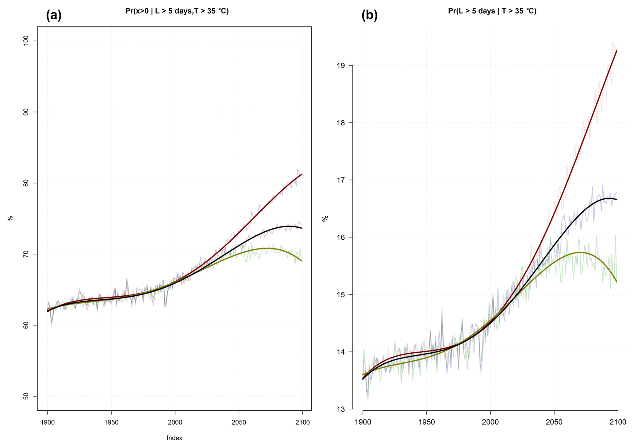
https://www.adv-stat-clim-meteorol-oceanogr.net/4/37/2018/ascmo-4-37-2018-f04

Figure 4Projected probability of (a) one or more events with daily maximum temperature above 35 ^∘C lasting longer than 5 days during the February–April season for Patna and (b) the probability that the heatwave lasts more than 5 days, given temperature above 35 ^∘C. These curves represent one of the stations presented in Tables 1 and 2. The fitted trend curves were fourth-order polynomials for different emission scenarios (Benestad, 2003), where green represents RCP2.6, blue RCP4.5, and red RCP8.5.

Download

Figure 4 shows for one selected location (Patna; row six in the table) (a) the probability of one or more heatwaves in a season and (b) the probability that a hot event lasts more than 5 days, based on the ensemble median of the downscaled projections for three different emission scenarios. Figure 5 presents the projected probabilities for 2100 assuming emission scenario RCP4.5 (the fourth columns in Tables 1 and 2) for all stations in India. According to the results presented in Fig. 4a, continuing global warming will imply an increased probability of long-lasting heatwaves in Patna, and Fig. 4b indicates that the likelihood for future 5-day heatwaves will depend on the future emissions, where the probability may increase by almost as much as a third from present-day values for the high-emission scenario: the probability of a 5-day or longer heatwave is approximately 15 % at the present time, but it is expected to increase to 19 % in 2100 in a continued high-emission scenario (RCP 8.5). For the intermediate-emission scenario RCP4.5, the results suggest an increase from 15 % to 17 % probability and an increase which is about half of that associated with RCP8.5. Hence, lower-emission scenarios give smaller increases. The maps presented in Fig. 5 suggest greater probabilities for heatwaves in the central parts of India. The variable skill of downscaling at different locations implies that the results are less accurate for some parts of India, namely the far eastern and southern parts.

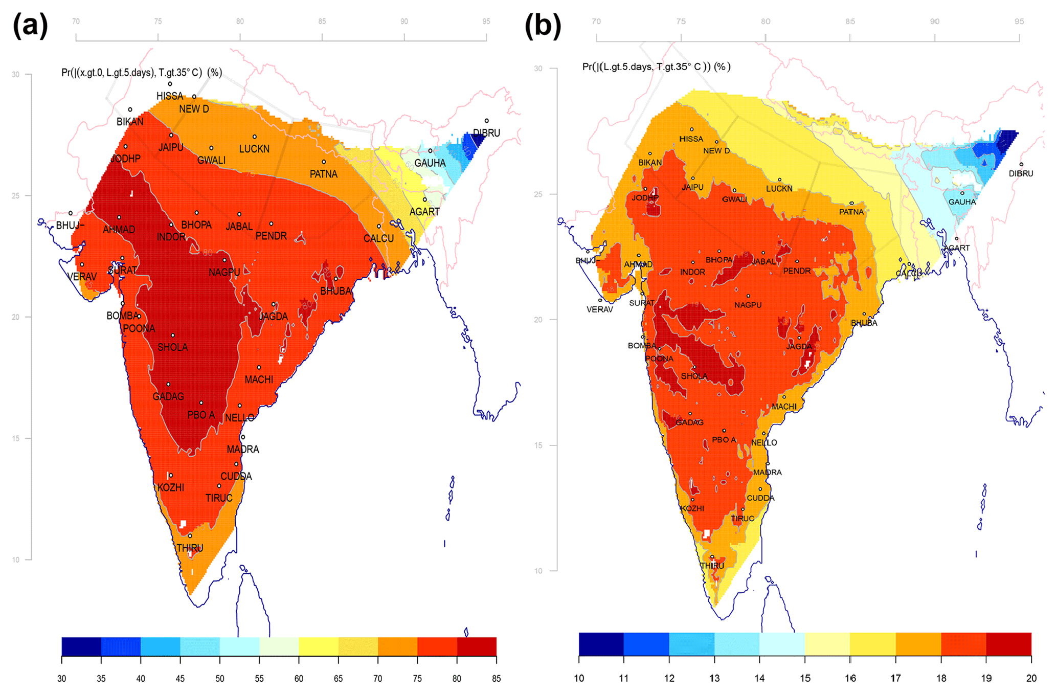
https://www.adv-stat-clim-meteorol-oceanogr.net/4/37/2018/ascmo-4-37-2018-f05

Figure 5Projected probability of (a) one or more events with daily maximum temperature above 35 ^∘C lasting longer than 5 days during the February–April season in 2100 assuming the RCP4.5 emission scenario and (b) the probability that the heat lasts longer than 5 days given a hot day in 2100 assuming the RCP4.5 emission scenario. The map was generated by gridding estimates shown in the fourth column in Table 1.

Download

4 Discussion

A number of studies suggest a more pronounced change in climatic extremes compared to changes in the mean (Colombo et al., 1999; Katz and Brown, 1992; Mearns et al., 1984; Meehl et al., 2000). The shape of the pdf for temperature may change with a shift in the mean μ, and the relationship between the mean and the shape of the pdf was tested on the actual temperature data used herein. A scatter plot between seasonal mean and seasonal standard deviation σ showed that it tends to decrease with increasing mean values (Supplement). Hence, since the mean often is not a good predictor for extreme values, we used the mean temperature to estimate the mean of another pdf; in this case, the seasonal mean daily maximum temperature was used to estimate the mean number of events and mean duration of heatwaves: $\overline{n_{5 d}} = f (\overline{T_{max}})$ and $\overline{L_{H}} = g (\overline{T_{max}})$ .

The analysis of the mean number of heatwaves lasting more than 5 days $\overline{n_{5 d}}$ and the mean duration of heatwaves had some caveats, and an assessment of the conformity of n_5 d to the normal distribution suggested divergence towards the tail of the distribution. One plausible reason for the deviation was that the mean was taken from small samples of Poisson-distributed data, whereas the mean was expected to converge to the normal distribution with large sample size. The divergence from the normal distribution may also have been a result of variable data quality. Nevertheless, using the mean duration and the mean number of events could justify using OLMs instead of GLMs since aggregated variables are expected to be closer to being normally distributed than the underlying data.

A more traditional approach is to downscale the temperature day by day, for instance through the means of regional climate models (RCMs), and then apply extreme-value theory to the model results. RCMs will not give a direct answer, as they have biases and suffer from other shortcomings. Hence, RCM-based studies also come with a set of uncertainties. However, there is a great benefit in having more than one approach as different strategies for estimating the results have different strengths and weaknesses independent of each other.

According to both Tables 1 and 2, the observed frequency of heatwaves was substantially lower than the estimated corresponding probability for seven sites in the far north-eastern parts of India or near India's western coast (Gauhati, Dibrugarh, Veraval, Kozhikode, Thiruvananthapuram, Bombay, Agartala), but for the 12 sites in interior parts of India where wheat is grown (the IGP region) and along India's east coast, they indicated a good match with a 25 % difference or smaller. All of these temperature records were deteriorated by missing data; to produce usable spell duration statistics, it was necessary to fill in short gaps of missing data by the means of linear interpolation. As the proportion of missing values was in the range of 7 %–34 %, the observed number of events in Tables 1 and 2 needs to be interpreted with caution. The sites with large mismatch were missing more than 15 % of values in their data record (Gauhati: 15.5 %; Dibrugarh: 34 %; Veraval: 19.5 %; Kozhikode: 23.5 %; Thiruvananthapuram: 24.6 %; Bombay: 18.4 %; Agartala: 22.6 %). A more detailed diagnostics of the data quality and the discrepancy between observed frequencies of heatwaves longer than 5 days and estimated likelihoods is provided in the Supplement, which suggests that the poor matches coincided with stations that carried low weights in the leading PCA. Some discrepancies between the downscaled probability and the observed frequency must also be expected since the former was based on a Bayesian-type analysis whereas the latter was based on observed counts. The bias in the estimated probability of a hot spell lasting more than 5 days compared to estimated frequency for the observations for the IGP region suggested that the estimates of probability type 2 may be less skillful than those of type 1. One reason may be that quality of the Indian data was low, which may be the reason for the differences in the scatter plots between $\overline{L_{H}}$ and $\overline{T_{max}}$ in India and Europe (Figs. 1b and 2 and Supplement). The hot spells were also not quite geometrically distributed (Fig. 3), which also could introduce an additional bias.

The question of the degree of validity of the relationship $\overline{L_{H}} = g (\overline{T_{max}})$ depends on the data quality and volume. While there was a weak link in India, there was a clear link over Europe. Furthermore, tests applied to ideal synthetic data indicated a connection between the two, and similar noisy scatter at the upper (lower for cold spells) tail of the ideal synthetic stochastic data ( $x \sim N (μ, σ^{2})$ ) in Fig. 1 suggested that estimates for more extreme cases were subject to increased sampling fluctuations. The noisy picture given by the scatter plots may also suggest that there were other unaccounted-for factors which influence the mean duration or the mean number of heatwaves. Another question is its validity in the future, as the connection may change if the shape of the pdf for T_max changes under global warming. The agreement between the link established for the European data and the ideal data (Fig. 1) suggests a universal trait as long as the daily temperature is approximately normally distributed, but a bias is likely to be present if the standard deviation diminishes (Supplement).

We wanted to demonstrate how this downscaling methodology makes the best use of the sketchy data, as the estimates themselves are based on more robust statistical parameters such as the mean duration $\overline{L_{H}}$ and the PCA of the mean temperature $\overline{T_{max}}$ . These quantities may be considered to be fairly resistant to errors as long as there are not too many of them, and that they are both random and unbiased. Furthermore, the PCA is resistant to errors in single temperature series as long as they represent a small number of the stations and are uncorrelated with errors at other sites. However, the interpolation of gaps with missing data introduced new uncertainties, and the presence of missing data also made it tricky to get accurate estimates for the heatwave durations. Missing data and errors introduced through interpolation represent one possible explanation for the poor match between the observed frequency of heatwaves in Table 2 and estimated likelihood for 5-day heatwaves at some of the sites. Moreover, the sites with the largest mismatch were not in regions where wheat crops are important, but we included them here to maximise the signal in the PCA and to enhance the chance of getting a good estimate of the dependency between large and small scales needed for empirical-statistical downscaling.

The analysis presented here was based on a novel methodology where the probability associated with heatwave duration was calculated from downscaled seasonal mean temperature estimates rather than inferring it from downscaled daily data. There has been some similar work, but none that have involved downscaling of large multi-model ensembles to make projections for heatwaves over India. Lana et al. (2008) did not include downscaling and used a Weibull distribution to describe the spell duration statistics rather than the geometric distribution. We chose the latter since it is based on the number of successive probabilities (hot days; see the Appendix). The analysis presented by Wang et al. (2015) was more similar to our projections of heatwave statistics over India, but they used bias-corrected GCM results for China rather than downscaling over India. We, on the other hand, combined statistical modelling of heatwave statistics with the empirical-statistical downscaling of February–April mean daily maximum temperature involving several multi-model ensembles.

The probabilities presented here were subject to a number of uncertainties: (a) the unknown nature of future emissions, (b) shortcomings in the global climate models, (c) limitations of the empirical-statistical downscaling method, (d) uncertainties associated with the connection between the mean daily maximum temperature and the duration statistics, and (e) errors in the observations. By including three different emission scenarios (RCPs 2.6, 4.5, and 8.5), the analysis provided some indication of the sensitivity of the probabilities to the nature of the emissions. Both Fig. 4 and Tables 1–2 indicate that future emissions mattered for the likelihood of longer lasting heatwaves, which have negative effects on wheat crops. Figures 1–3 present an evaluation of the connection between the mean daily maximum temperature and the heatwave duration statistics and reveal that it is not “perfect”, particularly for very long lasting heatwaves (>30 days). This connection nevertheless provides a reasonable estimate, and the comparison between synthetic normally distributed random data with similar autocorrelation suggested that this connection is robust. However, the connection would be sensitive to a change in the autocorrelation, although the autocorrelation appears to be insensitive to variations in physical conditions (Benestad et al., 2016).

It is impossible to predict the course of natural variability, and even a single climate model may produce different projections with widely different outcomes on local and regional scales (Deser et al., 2012). Probabilities account for such variability, and the analysis presented here made use of the median of the simulated temperature from large multi-model ensembles and a Bayesian-inspired approach to account for both natural variability and model differences. Such ensembles cannot be considered to be unbiased statistical samples (Benestad et al., 2017 b) as different models have similar biases since they share many components. The model differences, however, have been found to be less pronounced than the year-to-year variations (Benestad et al., 2016) and can for all intents and purposes be used as an imperfect description of the statistical spread when better information is lacking. The estimation of future probabilities also makes the question of statistical significance less relevant, since statistical significance refers to the probability that a change in a random variable is due to chance, assuming that the variable has a stochastic nature. In this case, the estimation of a change in probabilities is on the same level as the estimation of the probability levels commonly used in statistical significance tests.

5 Conclusions

We presented a case study for Indian wheat crops to test a methodology for estimating probabilities of long-lasting heatwaves, based on statistical modelling of streak lengths, their dependency on the seasonal mean of daily maximum temperature, and empirical-statistical downscaling of multi-model ensembles. Wheat crops appear to be subject to increased risks of heat stress in 2100 due to more frequent heatwaves with daily maximum temperature exceeding 35 ^∘C that last more than 5 days.

Code and data availability

Code for reproducing this experiment is provided in the Supplement as an R Markdown script (pdf and Rmd files). The data are freely available from figshare: https://figshare.com/articles/Heatwave_duration/5769345 (last access: 12 October 2018).

Appendix A: Method: details and code

The geometric distribution (Wilks, 1995) describes the probability distribution of the number X of Bernoulli trials needed to get one success, and Pr(X) can be defined according to

\begin{matrix} (A1) & Pr (X = k) = (1 - p)^{(k - 1)} p \forall k = {1, 2, 3, \dots}, \end{matrix}

where k is the number of days with heat and $p = 1 / \overline{L_{H}}$ is the probability of heat on any given day. There are two types of geometric distributions, and here we used the one describing number of failures before one success. Here the notation $\overline{X}$ is used to represent the mean value of a random daily variable X (temperature or heatwave length) over the February–April season. We used this equation to estimate the probability of the occurrence of heatwaves lasting more than 5 days, given an estimate for the mean duration of the spells: $Pr (L_{H} > 5 | \overline{L_{H}}) = [1 - Pr (L_{H} \leq 5 | \overline{L_{H}})] = [1 - \sum_{k = 1}^{5} Pr (X = k)]$ .

The probability based on the geometric distribution refers to a single heatwave event, and the probability of a long-lasting heatwave is higher with an increasing number of heatwaves. $\overline{L_{H}}$ depended on the mean temperature $\overline{T_{max}}$ and was modelled through GLMs that assumed a geometric or Poisson distribution. We also used downscaled $\overline{T_{max}}$ from multi-model ensembles to provide an ad hoc statistical distribution for the temperature and the ensemble median to specify a threshold for which the probability of higher temperature was 0.5.

The estimation of probabilities was based on

\begin{array}{l} Pr (L_{H} > 5 | \overline{T_{max}}) = \\ (A2) & Pr (L_{H} > 5 | \overline{L_{H}} (\overline{T_{max}})) Pr (\overline{T_{max}} > x), \end{array}

where $Pr (\overline{T_{max}} > x) = 1 / 2$ was represented by the 50th percentile of the multi-model ensemble. In the equation above, $Pr (L_{H} > 5 | \overline{L_{H}} (\overline{T_{max}}))$ represents the geometric distribution defined by parameter $p = 1 / \overline{L_{H}} (\overline{T_{max}}$ ), where $\overline{L_{H}}$ is a function of $\overline{T_{max}}$ and estimated though the GLM as shown in Fig. 2. In some cases, there may be several long-lasting events in a season; however, merely one is enough for negative impacts on the wheat crops.

We used a strategy described in Benestad et al. (2015 a) to fill gaps in seasonal mean aggregates of T_max and L_H, based on the function pcafill in the esd package. Interpolated values that were outside the original range of data were set to those maximum or minimum values.

The analysis was carried out in the R computing environment (R Core Team, 2014), and an R Markdown script with line-by-line instructions for the analysis carried out here is openly available from a GitHub repository (https://github.com/metno/esd_Rmarkdown/tree/master/CixPAG, last access: 21 September 2017). The analysis made use of the R package esd (Benestad et al., 2015 b).

Supplement

The supplement related to this article is available online at: https://doi.org/10.5194/ascmo-4-37-2018-supplement.

Author contributions

REB designed and carried out the analysis, whereas the co-authors contributed to writing the paper. JS is also the project leader of CixPAG.

Competing interests

The authors declare that they have no conflict of interest.

Acknowledgements

This work was funded by the Norwegian Research Council through the CixPAG project (grant number: 244551) and the Norwegian Meteorological Institute. Christian Wilhelm Mohr provided coordinates for the IGP region.

Edited by: Sarah Perkins-Kirkpatrick
Reviewed by: David Keellings and Yun Li

References

Asseng, S., Foster, I., and Turner, N.: The impact of temperature variability on wheat yields, Glob. Change Biol., 17, 997–1012, 2011. a

Asseng, S., Ewert, F., Martre, P., Rötter, R. P., Lobell, D. B., Cammarano, D., Kimball, B. A., Ottman, M. J., Wall, G. W., White, J. W., Reynolds, M. P., Alderman, P. D., Prasad, P. V. V., Aggarwal, P. K., Anothai, J., Basso, B., Biernath, C., Challinor, A. J., Sanctis, G. D., Doltra, J., Fereres, E., Garcia-Vila, M., Gayler, S., Hoogenboom, G., Hunt, L. A., Izaurralde, R. C., Jabloun, M., Jones, C. D., Kersebaum, K. C., Koehler, A.-K., Müller, C., Kumar, S. N., Nendel, C., O'Leary, G., Olesen, J. E., Palosuo, T., Priesack, E., Rezaei, E. E., Ruane, A. C., Semenov, M. A., Shcherbak, I., Stöckle, C., Stratonovitch, P., Streck, T., Supit, I., Tao, F., Thorburn, P. J., Waha, K., Wang, E., Wallach, D., Wolf, J., Zhao, Z., and Zhu, Y.: Rising temperatures reduce global wheat production, Nature Climate Change, 5, 143, https://doi.org/10.1038/nclimate2470, 2015. a

Barlow, K., Christy, B., O'Leary, G., Riffkin, P., and Nuttall, J.: Simulating the impact of extreme heat and frost events on wheat crop production: A review, Field Crop. Res., 171, 109–119, https://doi.org/10.1016/j.fcr.2014.11.010, 2015. a

Benestad, R.: Downscaling Climate Information, Oxford Research Encyclopedia of Climate Science, Oxford University Press, https://doi.org/10.1093/acrefore/9780190228620.013.27, 2016. a

Benestad, R.: Heatwave duration, https://doi.org/10.6084/m9.figshare.5769345.v2, 2018. a

Benestad, R., Parding, K., Dobler, A., and Mezghani, A.: A strategy to effectively make use of large volumes of climate data for climate change adaptation, Climate Services, 6, 48–54, https://doi.org/10.1016/j.cliser.2017.06.013, 2017a. a

Benestad, R., Sillmann, J., Thorarinsdottir, T. L., Guttorp, P., Mesquita, M. d. S., Tye, M. R., Uotila, P., Maule, C. F., Thejll, P., Drews, M., and Parding, K. M.: New vigour involving statisticians to overcome ensemble fatigue, Nature Climate Change, 7, 697–703, https://doi.org/10.1038/nclimate3393, 2017b. a, b

Benestad, R. E.: A comparison between two empirical downscaling strategies, Int. J. Climatol., 21, 1645–1668, https://doi.org/10.1002/joc.703, 2001. a

Benestad, R. E.: What can present climate models tell us about climate change?, Climatic Change, 59, 311–332, 2003. a

Benestad, R. E., Chen, D., Mezghani, A., Fan, L., and Parding, K.: On using principal components to represent stations in empirical-statistical downscaling, Tellus A, 67, 1, https://doi.org/10.3402/tellusa.v67.28326, 2015a. a, b

Benestad, R. E., Mezghani, A., and Parding, K. M.: esd V1.0, Zenodo, https://doi.org/10.5281/zenodo.29385, 2015b. a, b, c

Benestad, R. E., Parding, K. M., Isaksen, K., and Mezghani, A.: Climate change and projections for the Barents region: what is expected to change and what will stay the same?, Environ. Res. Lett., 11, 054017, https://doi.org/10.1088/1748-9326/11/5/054017, 2016. a, b, c, d, e, f, g

Chen, H., Xu, C.-Y., and Guo, S.: Comparison and evaluation of multiple GCMs, statistical downscaling and hydrological models in the study of climate change impacts on runoff, J. Hydrol., 434–435, 36–45, https://doi.org/10.1016/j.jhydrol.2012.02.040, 2012. a

Colombo, A. F., Etkin, D., and Karney, B. W.: Climate Variability and the Frequency of Extreme Temperature Events for Nine Sites across Canada: Implications for Power Usage, J. Climate, 12, 2490–2502, https://doi.org/10.1175/1520-0442(1999)012<2490:CVATFO>2.0.CO;2, 1999. a

Deser, C., Knutti, R., Solomon, S., and Phillips, A. S.: Communication of the role of natural variability in future North American climate, Nature Climate Change, 2, 775–779, 2012. a

Dobson, A.: An Introduction to Generalized Linear Models, Chapman and Hall, London, 1990. a

Duncan, J. M. A., Dash, J., and Atkinson, P. M.: Elucidating the impact of temperature variability and extremes on cereal croplands through remote sensing, Glob. Change Biol., 21, 1541–1551, https://doi.org/10.1111/gcb.12660, 2015. a

Furrer, E. M., Katz, R. W., Walter, M. D., and Furrer, R.: Statistical modeling of hot spells and heat waves, Clim. Res., 43, 191–205, https://doi.org/10.3354/cr00924, 2010. a, b, c

Gutiérrez, J. M., Maraun, D., Widmann, M., Huth, R., Hertig, E., Benestad, R., Roessler, O., Wibig, J., Wilcke, R., Kotlarski, S., Martín, D. S., Herrera, S., Bedia, J., Casanueva, A., Manzanas, R., Iturbide, M., Vrac, M., Dubrovsky, M., Ribalaygua, J., Pórtoles, J., Räty, O., Räisänen, J., Hingray, B., Raynaud, D., Casado, M. J., Ramos, P., Zerenner, T., Turco, M., Bosshard, T., Štěpánek, P., Bartholy, J., Pongracz, R., Keller, D. E., Fischer, A. M., Cardoso, R. M., Soares, P. M. M., Czernecki, B., and Pagé, C.: An intercomparison of a large ensemble of statistical downscaling methods over Europe: Results from the VALUE perfect predictor cross-validation experiment, Int. J. Climatol., https://doi.org/10.1002/joc.5462, online first, 2018. a

Hansen, B. B., Isaksen, K., Benestad, R. E., Kohler, J., Pedersen, A. Ø., Loe, L. E., Coulson, S. J., Larsen, J. O., and Varpe, Ø.: Warmer and wetter winters: characteristics and implications of an extreme weather event in the High Arctic, Environ. Res. Lett., 9, 114021, https://doi.org/10.1088/1748-9326/9/11/114021, 2014. a

Hatfield, J. L. and Prueger, J. H.: Temperature extremes: Effect on plant growth and development, Weather and Climate Extremes, 10, 4–10, https://doi.org/10.1016/j.wace.2015.08.001, 2015. a

Iizumi, T. and Ramankutty, N.: How do weather and climate influence cropping area and intensity?, Glob. Food Secur.-Agr., 4, 46–50, https://doi.org/10.1016/j.gfs.2014.11.003, 2015. a

Kahneman, D.: Thinking, Fast and Slow, Penguin, London, 2012. a

Katz, R. W. and Brown, B. G.: Extreme events in a changing climate: Variability is more important than averages, Climatic Change, 21, 289–302, https://doi.org/10.1007/BF00139728, 1992. a

Keellings, D. and Waylen, P.: Increased risk of heat waves in Florida: Characterizing changes in bivariate heat wave risk using extreme value analysis, Appl. Geogr., 46, 90–97, https://doi.org/10.1016/j.apgeog.2013.11.008, 2014. a, b

Klein Tank, A. J. B. W., Konnen, G. P., Böhm, R., Demarée, G., Gocheva, A., Mileta, M., Pashiardis, S., Hejkrlik, L., Kern-Hansen, C., Heino, R., Bessemoulin, P., Müller-Westermeier, G., Tzanakou, M., Szalai, S., Pálsdóttir, T., Fitzgerald, D., Rubin, S., Capaldo, M., Maugeri, M., Leitass, A., Bukantis, A., Aberfeld, R., Engelen, A. F. V. v., Forland, E., Mietus, M., Coelho, F., Mares, C., Razuvaev, V., Nieplova, E., Cegnar, T., López, J. A., Dahlström, B., Moberg, A., Kirchhofer, W., Ceylan, A., Pachaliuk, O., Alexander, L. V., and Petrovic, P.: Daily dataset of 20th-century surface air temperature and precipitation series for the European Climate Assessment, Int. J. Climatol., 22, 1441–1453, 2002. a, b

Koehler, A.-K., Challinor, A. J., Hawkins, E., and Asseng, S.: Influences of increasing temperature on Indian wheat: quantifying limits to predictability, Environ. Res. Lett., 8, 034016, https://doi.org/10.1088/1748-9326/8/3/034016, 2013. a

Krishnan, M., Nguyen, H. T., and Burke, J. J.: Heat shock protein synthesis and thermal tolerance in wheat, Plant Physiol., 90, 140–145, 1989. a

Kumar, K. K., Rajagopalan, B., Hoerling, M., Bates, G., and Cane, M.: Unraveling the Mystery of Indian Monsoon Failure During El Nino, Science, 314, 115–119, https://doi.org/10.1126/science.1131152, 2006. a

Lana, X., Martínez, M. D., Burgueño, A., Serra, C., Martín-Vide, J., and Gómez, L.: Spatial and temporal patterns of dry spell lengths in the Iberian Peninsula for the second half of the twentieth century, Theor. Appl. Climatol., 91, 99–116, https://doi.org/10.1007/s00704-007-0300-x, 2008. a, b

Lobell, D., Sibley, A., and Ortiz-Monasterio, J.: Extreme heat effects on wheat senescence in India, Nature Climate Change, 2, 186–189, https://doi.org/10.1038/nclimate1356, 2012a. a

Lobell, D. B., Sibley, A., and Ivan Ortiz-Monasterio, J.: Extreme heat effects on wheat senescence in India, Nature Climate Change, 2, 186–189, https://doi.org/10.1038/nclimate1356, 2012b. a, b

Luo, Q.: Temperature thresholds and crop production: a review, Climatic Change, 109, 583–598, 2011a. a

Luo, Q.: Temperature thresholds and crop production: a review, Temperature thresholds and crop production: a review, Climatic Change, 109, 583–598, https://doi.org/10.1007/s10584-011-0028-6, 2011b. a

Maraun, D., Wetterhall, F., Ireson, A. M., Chandler, R. E., Kendon, E. J., Widmann, M., Brienen, S., Rust, H. W., Sauter, T., Themeßl, M., Venema, V. K. C., Chun, K. P., Goodess, C. M., Jones, R. G., Onof, C., Vrac, M., and Thiele-Eich, I.: Precipitation downscaling under climate change: Recent developments to bridge the gap between dynamical models and the end user, Rev. Geophys., 48, RG3003, https://doi.org/10.1029/2009RG000314, 2010. a

McCullagh, P. and Nelder, J.: Generalized Linear Models, Chapman and Hall, London, 1989. a

McMaster, G. S., White, J. W., Hunt, L. A., Jamieson, P. D., Dhillon, S. S., and Ortiz-Monasterio, J. I.: Simulating the Influence of Vernalization, Photoperiod and Optimum Temperature on Wheat Developmental Rates, Simulating the Influence of Vernalization, Photoperiod and Optimum Temperature on Wheat Developmental Rates, Ann. Bot., 102, 561–569, https://doi.org/10.1093/aob/mcn115, 2008. a

Mearns, L. O., Katz, R. W., and Schneider, S. H.: Extreme High-Temperature Events: Changes in their probabilities with Changes in Mean Temperature, J. Clim. Appl. Meteorol., 23, 1601–1613, https://doi.org/10.1175/1520-0450(1984)023<1601:EHTECI>2.0.CO;2, 1984. a

Meehl, G. A., Zwiers, F., Evans, J., Knutson, T., Mearns, L., and Whetton, P.: Trends in Extreme Weather and Climate Events: Issues Related to Modeling Extremes in Projections of Future Climate Change, B. Am. Meteorol. Soc., 81, 427–436, https://doi.org/10.1175/1520-0477(2000)081<0427:TIEWAC>2.3.CO;2, 2000. a

Menne, M. J., Durre, I., Korzeniewski, B., McNeill, S., Thomas, K., Yin, X., Anthony, S., Ray, R., Vose, R. S., Gleason, B. E., and Houston, T. G.: Global Historical Climatology Network – Daily (GHCN-Daily), Version 3, NOAA National Climatic Data Center, 2012a. a

Menne, M. J., Durre, I., Vose, R. S., Gleason, B. E., and Houston, T. G.: An Overview of the Global Historical Climatology Network-Daily Database, J. Atmos. Ocean. Tech., 29, 897–910, https://doi.org/10.1175/JTECH-D-11-00103.1, 2012b. a

Mishra, S. C., Singh, S. K., Patil, R., Bhusal, N., Malik, A., and Sareen, S.: Breeding for heat tolerance in Wheat, in: WHEAT: Recent Trends on Production Strategies of Wheat in India, edited by: Shukla, R. S., Mishra, P. C., Chatrath, R., Gupta, R. K., Tomar, S. S., and Sharma, I., 15–29, DWR, Karnal, 2014. a

Neumann, J. and Kington, J.: Great Historical Events That Were Significantly Affected by the Weather: Part 10, Crop Failure in Britain in 1799 and 1800 and the British Decision to Send a Naval Force to the Baltic Early in 1801, B. Am. Meteorol. Soc., 73, 187–199, https://doi.org/10.1175/1520-0477(1992)073<0187:GHETWS>2.0.CO;2, 1992. a

Nychka, D.: LatticeKrig: A multi-resolution spatial model for large data., in: Spatial Statistics for Environmental and Energy Challenges – Workshop 2014, Thuwal, Saudi Arabia, 2014. a

Porter, J. R. and Gawith, M.: Temperatures and the growth and development of wheat: a review, Eur. J. Agron., 10, 23–36, 1999. a, b

Rao, B. B., Chowdary, P. S., Sandeep, V., Pramod, V., and Rao, V.: Spatial analysis of the sensitivity of wheat yields to temperature in India, Spatial analysis of the sensitivity of wheat yields to temperature in India, Agr. Forest Meteorol., 200, 192–202, https://doi.org/10.1016/j.agrformet.2014.09.023, 2015. a, b, c

R Core Team: R: A Language and Environment for Statistical Computing, R Foundation for Statistical Computing, Vienna, Austria, 2014. a

Saini, H. and Aspinall, D.: Abnormal sporogenesis in wheat (Triticum aestivum L.) induced by short periods of high temperature, Ann. Bot., 49, 835–846, 1982. a, b

Saxena, D. C., Prasad, S. V. S., Parashar, R., and Rathi, I.: Phenotypic characterization of specific adaptive physiological traits for heat tolerance in wheat, Phenotypic characterization of specific adaptive physiological traits for heat tolerance in wheat, Indian J. Plant Physi., 21, 318–322, https://doi.org/10.1007/s40502-016-0241-4, 2016. a

Schubert, S.: Downscaling local extreme temperature change in south-eastern Australia from the CSIRO MARK2 GCM, Int. J. Climatol., 18, 1419–1438, 1998. a

Sharma, S., Sharma, R., and Chaudhary, H.: Vernalization response of winter x spring wheat derived doubled-haploids, Vernalization response of winter x spring wheat derived doubled-haploids, Afr. J. Agr. Res., 7, 6465–6473, https://doi.org/10.5897/AJAR12.2114, 2012. a

Simmons, A. and Gibson, J.: The ERA-40 Project Plan, ERA-40 Project Report Series 1, ECMWF, available at: https://www.ecmwf.int/ (last access: 23 April 2018), 2000. a

Sivakumar, M. V. K.: Empirical Analysis of Dry Spells for Agricultural Applications in West Africa, J. Climate, 5, 532–539, https://doi.org/10.1175/1520-0442(1992)005<0532:EAODSF>2.0.CO;2, 1992. a

Storch, H. v., Zorita, E., and Cubasch, U.: Downscaling of Global Climate Change Estimates to Regional Scales: An Application to Iberian Rainfall in Wintertime, J. Climate, 6, 1161–1171, 1993. a

Tashiro, T. and Wardlaw, I.: The response to high temperature shock and humidity changes prior to and during the early stages of grain development in wheat, Funct. Plant Biol., 17, 551–561, 1990. a, b

Tiwari, V., Mamrutha, H. M., Sareen, S., Sheoran, S., Tiwari, R., Sharma, P., Singh, C., Singh, G., and Rane, J.: Managing Abiotic Stresses in Wheat, in: Abiotic Stress Management for Resilient Agriculture, edited by: Minhas, P., Rane, J., and Pasala, R., 313–337, Springer, Singapore, https://doi.org/10.1007/978-981-10-5744-1_14, 2017. a

Wang, W., Zhou, W., Li, Y., Wang, X., and Wang, D.: Statistical modeling and CMIP5 simulations of hot spell changes in China, Clim. Dynam., 44, 2859–2872, https://doi.org/10.1007/s00382-014-2287-1, 2015. a, b, c

Wilby, R. and Wigley, T.: Downscaling General Circulation Model output: a review of methods and limitations, Prog. Phys. Geogr., 21, 530–548, 1997. a

Wilks, D. S.: Statistical Methods in the Atmospheric Sciences, Academic Press, Orlando, Florida, USA, 1995. a, b

Xue, G.-P., Sadat, S., Drenth, J., and McIntyre, C. L.: The heat shock factor family from Triticum aestivum in response to heat and other major abiotic stresses and their role in regulation of heat shock protein genes, J. Exp. Bot., 65, 539–557, 2013. a

Articles

Short summary

A new study indicates that heatwaves in India will become more frequent and last longer with global warming. Its results were derived from a large number of global climate models, and the calculations differed from previous studies in the way they included advanced statistical theory. The projected changes in the Indian heatwaves will have a negative consequence for wheat crops in India.